tasks such as optical music recognition (OMR), is much more challenging than ... Otsu (1979), Lloyd (1985), Kittler and Illingworth (1986),. Yanni and Horne ...
A COMPARATIVE SURVEY OF IMAGE BINARISATION ALGORITHMS FOR OPTICAL RECOGNITION ON DEGRADED MUSICAL SOURCES John Ashley Burgoyne Laurent Pugin Greg Eustace Ichiro Fujinaga Centre for Interdisciplinary Research in Music and Media Technology Schulich School of Music of McGill University Montr´eal, Qu´ebec, Canada H3A 1E3 {ashley,laurent,greg,ich}@music.mcgill.ca ABSTRACT Binarisation of greyscale images is a critical step in optical music recognition (OMR) preprocessing. Binarising music documents is particularly challenging because of the nature of music notation, even more so when the sources are degraded, e.g., with ink bleed-through from the other side of the page. This paper presents a comparative evaluation of 25 binarisation algorithms tested on a set of 100 music pages. A real-world OMR infrastructure for early music (Aruspix) was used to perform an objective, goaldirected evaluation of the algorithms’ performance. Our results differ significantly from the ones obtained in studies on non-music documents, which highlights the importance of developing tools specific to our community. 1 INTRODUCTION Binarising music documents, that is separating the foreground from the background in order to prepare for other tasks such as optical music recognition (OMR), is much more challenging than binarising text documents. In text documents, the letters are all of approximately the same size and are regularly and uniformly distributed throughout the page. Music symbols, on the other hand, exhibit a wide range of sizes and markedly uneven distribution: they are clustered around musical staves. Large black areas, such as note heads, are conducive to ink accumulation during printing, which often results in strong bleedthrough (elements from the verso visible through the paper), especially for early sources. Large blank areas without foreground elements can disturb some binarisation techniques because bleed-through is often considered to be foreground. We will show in this paper that because of these conditions, the most widely used binarisation methods fail to produce suitable results for OMR. Evaluating the performance of binarisation algorithms is a difficult task. Very often, due to a lack of any evaluation infrastructure, researchers use subjective approaches, e.g., marking output as “better”, “same” or “worst” [3, 4]. When the binarisation is performed for the purpose of further image processing tasks, such as optical character c 2007 Austrian Computer Society (OCG).
recognition (OCR) or OMR, it makes more sense to use an objective evaluation. Evaluating the algorithms within the context of a real-world application enables goal-directed evaluation, which rates a binarisation algorithm on its ability to improve the post-binarisation task [10]. Furthermore, it has been shown that when document images have graphical particularities like music documents do, the use of goal-directed evaluation can lead to significant performance improvements [7]. 2 METHODS For our experiments, we used Aruspix, a software application for OMR on early music prints [7]. We selected five 16th-century music books (RISM 1520-2, 1532-10, 15385, M-0579 and M-0582 [8]) that suffer from severe degradation and transcribed 20 pages from each (100 total) to obtain ground-truth data for the evaluation. We tested 25 different binarisation algorithms over a range of parameters, which resulted in a set of 8,000 images. The images were deskewed and normalised to a consistent staff height (100 pixels) by Aruspix before applying the binarisation algorithm, and after binarisation, Aruspix was used again for the OMR evaluation. Binarisation methods can be categorised according to differences in the criteria used for thresholding. Sezgin and Sankur have proposed a taxonomy of thresholding techniques, including those based on the shape of the greyvalue histogram, measurement-space clustering, image entropy, connected-component attributes, spatial correlation, and the properties of a small, local windows around each pixel [9]. We chose a range of top-performing algorithms for both document images and what Sezgin and Sankur call non-destructive testing (NDT) images, which have more photo-like qualities; for the reasons mentioned above, music documents would be expected to fall somewhere between these two extremes. Methods based on histogram shape include those proposed by Sezan (1985) and Ramesh et al. (1995). Popular measurement-space clustering methods include those proposed by Ridler and Calvard (1978), Otsu (1979), Lloyd (1985), Kittler and Illingworth (1986), Yanni and Horne (1994), and Jawahar et al. (1997). Some entropy-based methods, also popular, are those of Dunn et al. (1984), Kapur et al. (1985), Li and Lee (1993), Shanbhag
(a) RISM 1520-2
(b) RISM 1538-5
(c) RISM M-0582
Figure 1. Three sample images from the test set.
(a) Brink and Pendock 1996
(b) Gatos et al. 2004
(c) Otsu 1979
Figure 2. Binarisation output from three algorithms on RISM 1538-5.
Algorithm Brink and Pendock 1996 Pugin 2007 Gatos et al. 2004 Sezan 1985 Li and Lee 1993 Pikaz and Averbuch 1996 Mardia and Hainsworth 1988 Yanowitz and Bruckstein 1989 Bernsen 1986 Niblack 1986 Yanni and Horne 1994 Otsu 1979 Ridler and Calvard 1978 Lloyd 1985 Kittler and Illingworth 1986 Jawahar et al. 1997 Ramesh et al. 1995 Sauvola and Pietaksinen 2000 Shanbhag 1994 Kapur et al. 1985 Abutaleb 1989 Leung and Lam 1998 White and Rohrer 1983 Yen et al. 1995 Dunn et al. 1984
Win.
21
17 31
31
15
Rate 79.2 78.2 76.4 76.4 75.9 72.9 72.1 68.9 67.0 66.7 63.3 62.7 62.3 60.2 58.2 57.3 56.0 55.5 53.2 43.4 39.9 37.6 36.5 23.7 2.7
Recall Odds multiplier 1.00 – 0.94 (0.89, 0.98) 0.84 (0.80, 0.88) 0.84 (0.80, 0.88) 0.82 (0.78, 0.86) 0.68 (0.65, 0.71) 0.66 (0.63, 0.69) 0.56 (0.53, 0.58) 0.51 (0.49, 0.53) 0.50 (0.48, 0.52) 0.42 (0.41, 0.44) 0.41 (0.40, 0.43) 0.40 (0.39, 0.42) 0.37 (0.35, 0.38) 0.34 (0.32, 0.35) 0.32 (0.31, 0.34) 0.31 (0.29, 0.32) 0.30 (0.29, 0.31) 0.28 (0.27, 0.29) 0.18 (0.17, 0.19) 0.15 (0.15, 0.16) 0.14 (0.13, 0.14) 0.13 (0.12, 0.14) 0.07 (0.06, 0.07) 0.01 (0.01, 0.01)
Rate 80.6 79.5 76.8 77.5 77.0 74.1 74.1 68.9 67.6 66.8 65.3 64.6 64.2 62.7 60.4 60.5 59.4 58.4 60.9 51.4 45.1 53.0 42.0 41.5 13.2
Precision Odds multiplier 1.00 – 0.92 (0.88, 0.97) 0.77 (0.74, 0.81) 0.82 (0.78, 0.86) 0.79 (0.76, 0.83) 0.67 (0.64, 0.70) 0.67 (0.64, 0.70) 0.51 (0.48, 0.53) 0.47 (0.45, 0.50) 0.45 (0.43, 0.47) 0.42 (0.41, 0.44) 0.41 (0.39, 0.43) 0.40 (0.39, 0.42) 0.37 (0.36, 0.39) 0.34 (0.32, 0.35) 0.34 (0.33, 0.36) 0.32 (0.31, 0.34) 0.30 (0.29, 0.32) 0.36 (0.34, 0.37) 0.23 (0.22, 0.24) 0.17 (0.17, 0.18) 0.24 (0.23, 0.25) 0.15 (0.14, 0.16) 0.15 (0.14, 0.16) 0.03 (0.03, 0.03)
Table 1. Overall results. All window-based algorithms are evaluated at their best window size. In addition to general recall and precision rates, more precise estimates of the odds multipliers and their 95% confidence intervals are given.
Figure 3. Recognition performance (recall) of Gatos et al. 2004, the top-performing window-based local binarisation algorithm, on each of the books in the test set. Note that there is no one optimal threshold. (1994), Yen et al. (1995), and Brink and Pendock (1996). We chose two object attribute methods, Pikaz and Averbuch (1996) and Leung and Lam (1998), and one spatial information method, Abutaleb (1989). Local thresholding techniques, which rely on the properties of a small window surrounding each pixel are commonly used despite their computational expense; we chose the methods of White and Rohrer (1983), Bernsen (1986), Niblack (1986), Mardia and Hainsworth (1988), Yanowitz and Bruckstein (1989), Sauvola and Pietaksinen (2000), and Gatos et al. (2004). Full references for these algorithms may be found in [1, 2, 9]. Finally, we developed a new algorithm that considers binarisation to be not a 2-class but a 3-class, foreground–bleed-through–background problem [6]. 3 RESULTS Although there is no standard metric for performance in OMR, Aruspix provides symbol-level recall and precision rates, as is standard in speech recognition and many other tasks in information retrieval. The appropriate statistical tool for analysing precision and recall across a data set is binomial regression, also known as logistic regression. The regression parameters are best interpreted as odds multipliers relative to some baseline such as a wellknown or high-performing algorithm [5]. In this paper, we have taken the baseline to be the performance of our best algorithm, which means that the odds multipliers range conveniently from 0 to 1 and represent the fraction of best possible performance one can expect from an algorithm. Before assessing performance across the data set, we needed to find the best window sizes for the locally adaptive algorithms. Previous work had suggested that the ideal region size was between 8 and 32 pixels for nor-
Figure 4. Recognition performance (recall) of all algorithms across the entire test set. One can see that the best algorithms perform fairly consistently while the poor algorithms lack consistency.
malised staves, or between 1/2 and 11/2 staff spaces [7]. Somewhat surprisingly, we found that there is no optimal region size. Figure 3, for example, shows the recognition performance of Gatos et al. 2004 for each book in the test set. For two books, the performance increases with window size for a time and then plateaus. For two others, the performance peaks at a window size of about 18 pixels and begins to decrease significantly as window size increases further. If binarisation had to be performed before staff recognition, tuning this parameter would be even more difficult if not impossible. Despite their advantages on manuscripts with markedly uneven (or stained) background, there is good reason to seek non-parametric alternatives to these locally adaptive algorithms. Fortunately, there are a number of non-parametric algorithms that perform much better than the window-based set. Table 1 presents a complete list of the performance of all algorithms. It is divided into the two traditional metrics of recall, or the percentage of symbols on the page that were found during the OMR process, and precision, or the percentage of symbols in the OMR output that were in fact on the page. In addition to overall recall and precision rates, we present the odds multiplier scores, which are a much more accurate means of comparing the algorithms. The odds multipliers are presented along with
their 95-percent confidence intervals to enable the reader to identify where the rankings are statistically significant and where they represent clusters. Wherever the confidence intervals are separated, e.g., between Niblack 1986, with a low point of 0.48, and Yanni and Horne, with a high point of 0.44, the difference is statistically significant. Table 1 is ordered by recall performance, which is the most important measure to optimise when trying to reduce human editing costs after the OMR process. The clear winner is Brink and Pendock 1996, which performs significantly better than all others in both performance and recall; a sample of its output appears in figure 2a. The new Pugin 2007 algorithm is a close second. The only locally adaptive algorithm to perform well was Gatos et al. 2004 (see figure 2b), a variant of Niblack 1986 that has been designed especially to treat document degradation. There is a large and significant performance gap in both recall and precision after Li and Lee 1993, which suggests that OMR researchers should concentrate their efforts on the top five algorithms in the table. None of them has received much attention to date, and indeed, the most commonly used binarisation algorithm is the notably mediocre Otsu 1979 (see figure 2c). A more visual representation of some of the data in Table 1 appears in figure 4. This figure is a box-andwhisker plot on recall performance for every image in the test set. The whiskers extend to the maximum and minimum performance for each algorithm, excepting cases where the performance is so high or low that it should be considered an unrepresentative outlier. These outliers are marked with small crossed boxes and tend to occur for the most difficult images in the set. The open white rectangles, which range from the first to third quartiles, give a visual cue to the amount of variance in each algorithm, and the line in the centre of each box denotes median performance. The most interesting aspect of this diagram is that the difference among these algorithms is not their best performance, which is acceptable for almost all of them, but rather their consistency of performance. The algorithms that rank poorly overall do so because their performance is widely variable, which puts undue pressure on the OMR process and makes quality control difficult. The best algorithms, in contrast, perform well not just on average but consistently almost all the time. As mentioned earlier, we selected these 24 algorithms in particular because they have historically performed well on either or both of document and NDT images. Our results, however, differ considerably from Sezgin and Sankur’s evaluations on these two classes of algorithms. Brink and Pendock 1996, for example, is only an average performer on Sezgin and Sankur’s document images and the worst performer on NDT images. Sauvola and Pietksinen 2000 and Kittler and Illingworth 1986, in contrast, are Sezgin and Sankur’s top performers for document images whereas they only obtain recall scores of 0.34 and 0.30 here. These differences confirm the special nature of musical documents and the necessity of developing a distinct set of image processing techniques for them.
4 SUMMARY AND FUTURE WORK Using a quantitative, goal-directed evaluation technique, we have performed an analysis of unprecedented scope for OMR. The project synthesises the most important surveys of image binarisation techniques and supplements them with the most recent work in the field. The results demonstrate the value of music-specific methods for image processing and provide a music-specific performance reference for the most successful binarisation algorithms in the field. The particular success of the three-class model in Pugin 2007 suggests that the other best-performing algorithms could be adapted fruitfully to improve their performance still further on documents suffering from difficult bleed-through. 5 ACKNOWLEDGEMENTS We would like to thank the Canada Foundation for Innovation and the Social Sciences and Humanities Research Council of Canada for their financial support. 6 REFERENCES [1] S. Bøe, “XITE – X-based image processing tools and environment – Reference manual for version 3.45,” Image Processing Laboratory, Dept. of Informatics, Univ. of Oslo, Tech. Rep., September 2004. [2] B. Gatos, I. Pratikakis, and S. J. Perantonis, “An adaptive binarisation technique for low quality historical documents,” in Proc. 6th Int. Work. Doc. Anal. Sys., pp. 102–13. [3] E. Kavallieratou and E. Stamatatos, “Adaptive binarization of historical document images,” in Proc. 18th Int. Conf. Pat. Rec., pp. 742–45. [4] G. Leedham, S. Varma, A. Patankar, and V. Govindarayu, “Separating text and background in degraded document images – a comparison of global threshholding techniques for multi-stage threshholding,” in Proceedings of the Eighth International Workshop on Frontiers in Handwriting Recognition (IWFHR’02), 2002. [5] P. McCullagh and J. A. Nelder, Generalized Linear Models, 2nd ed. London: Chapman and Hall, 1989. [6] L. Pugin, “A new binarisation algorithm for documents with bleed-through,” McGill University, Montreal, Tech. Rep. MUMT-DDMAL-07-01, March 2007. [7] L. Pugin, J. A. Burgoyne, and I. Fujinaga, “Goal-directed evaluation for the improvement of optical music recognition on early music prints,” in Proc. ACM/IEEE Joint Conf. Digital Libraries, Vancouver, Canada, 2007, pp. 303–04. [8] R´epertoire international des sources musicales (RISM), Single Prints Before 1800, ser. Series A/I. Kassel: B¨arenreiter, 1971–81. [9] M. Sezgin and B. Sankur, “Survey over image thresholding techniques and quantitative performance evaluation,” Journal of Electronic Imaging, vol. 13, no. 1, pp. 146–65, 2004. [10] Ø. D. Trier and A. K. Jain, “Goal-directed evaluation of binarization methods,” IEEE Transactions on PAMI, vol. 17, no. 12, pp. 1191–1201, 1995.