Article Submitted to :
A Comparison between Standard Bootstrap and Theiler’s Surrogate Methods M ELVIN J. H INICH∗1 , E DUARDO M. A. M. M ENDES†2
AND
L. S TONE‡3
1 Applied
Research Laboratories, University of Texas at Austin, Austin TX 78713-8029 USA de Engenharia Eletrônica, Universidade Federal de Minas Gerais, Av. Antônio Carlos 6627, Belo Horizonte, MG, Brazil, 31.270-901, Tel: +55 (31) 3449 4862, Fax: +55 (31) 3449 4850 3 Biomathematics Unit, Porter Super center for Ecological and Environmental Studies, Tel Aviv University, 69978, Israel.
2 Departamento
Abstract The Theiler method of surrogate data has been widely used for testing for the presence of nonlinearity in time series. Yet the Theiler surrogate method has not been applied in nonlinear time series in economics as yet. Economic and other social systems are nonlinear. Testing for the presence of nonlinearity is a first step in determining if a linear model is valid. Several tests for nonlinearity were compared by [W. Barnett et al., 1997]. One of the various tests for nonlinearity in their paper was a bootstrapped method by D. Kaplan that is an extension of the surrogate bootstrap pioneered by J. Theiler et al. [1992]. A comparison is made between this method and two other standard bootstrapping methods for generating false alarm rates and confidence intervals required for statistical hypothesis testing. Surrogate data bootstrapping has been widely used in the physical sciences literature dealing with nonlinearity in signals. We compare this method with standard Efron bootstrapping method and the shuffle bootstrap for generating sizes of tests that the higher order standardized cumulants are equal to their theoretical values for a normal, uniform, and exponential density. We also compare confidence intervals for the estimates of the standardized cumulants. As a conclusion the Theiler surrogate method is shown to be worthless if the null hypothesis is that the time series is a linear stochastic process that is not constrained to be a normal (gaussian) process. Yet Theiler’s method is not well behaved even if the null hypothesis is linear and normal.
1. Introduction Economic and other social systems are nonlinear. If the nonlinearity in the system is small then a linear approximation can yield good forecasts once the system parameters are estimated. But it the nonlinearity is large then a forecast based on an estimated linear approximation will be erroneous when the system changes paths. ∗ E-mail:
[email protected]
† E-mail:
[email protected]
‡ E-mail:
[email protected]
1
M. J. Hinich, E. Mendes and L. Stone: A comparison between Standard Bootstrap and
2
Testing for the presence of nonlinearity is a first step in determining if a linear model is valid. Several tests for nonlinearity were compared by W. Barnett et al. [1997]. One of the various tests for nonlinearity in their paper was a bootstrapped method by D. Kaplan that is an extension of the surrogate bootstrap pioneered by J. Theiler et al. [1992]. The “surrogate” approach is a resampling method that has been widely applied in the physics literature to test whether an observed time-series is consistent with the null hypothesis that the process is linear and normal. The Efron bootstrap [B. Efron, 1979a,b, B. Efron and R. Tibshirani, 1986, 1993] resampling method for determining critical regions or confidence intervals can not be directly applied to time series analysis due to the serial dependence in the stochastic process under analysis. The Theiler surrogate method is explained in the next several paragraphs, along with its fundamental weakness. The core weakness is the fact that most random processes in nature are not normal. The correct for null hypothesis tests of normality is that the process is linear. The normal component in the Theiler approach confounds its value. A linear non-normal process will be treated as if it were nonlinear. A linear discrete-time process is a linear combination of i.i.d random variables where the linear weights are absolutely summable. This sequence of weights is called a linear filter in the engineering science literature, which also uses the term gaussian rather than normal. For example x(tn ) = e(tn ) + 0.5e(tn − 1) is a linear process if the sequence e(tn ) is independently and identically distributed for times tn = nτ where τ is the sampling interval. If e(tn ) has a normal (gaussian) distribution then the process is called linear and normal (gaussian) and is abbreviated as LGP. We show in this paper that the application of the Central Limit Theorem implies that the Theiler surrogates are only consistent for the LGP null hypothesis. The surrogates are worthless if the null hypothesis is widened to the class of nonlinear stochastic processes. We present artificial data results to compare the Theiler surrogates with the Efron bootstraps for null hypotheses that the sample cumulants from three standard densities are equal to their theoretical values. We then compare the Efron bootstrapped confidence intervals with confidence intervals based on surrogates. Consider an observed sample time series x(t1 ), . . . , x(tN ). The discrete Fourier transform (DFT) of this sample is for k = 1, . . . , N − 1 tN
A( fk ) =
∑ x(tn)e−i2π fktn
(1)
n=t1
k is the k-th Fourier frequency. In polar form A( fk ) = |A( fk )|eiφ( fk ) where φ( fk ) is called the where fk = Nτ phase of A( fk ). Since the process is real A( fN−k ) = A∗ ( fk ) and φ(0) = 0. As long as the process satisfies a standard mixing condition such as the summable cumulants condition of Brillinger [1975], the phases are asymptotically independent uniform (−π, π) random variables. The Theiler method generates replicates called “surrogates” by replacing the true phases with a set of pseudo independent distributed uniform (−π, π) generated by any good pseudorandom uniform subroutines. The main objective is to provide a kind of baseline or control against which the original data can be compared. Letting µ( f1 ), . . . , µ( fN−1 ), where µ( fN−k ) = −µ( fk ) denote the pseudorandom phase, the surrogate is at time tn
x(t ˜ n) =
1 N−1 |A( fk )|ei2π fk µ(tk ) ∑ N k=0
(2)
M. J. Hinich, E. Mendes and L. Stone: A comparison between Standard Bootstrap and
3
As many surrogates is needed is generated by this method. Since expression 2 is a linear combination of independent variates with finite weights, the standard limit theorem implies that each surrogate has an approximate normal distribution. The physical idea behind the surrogates method is that a nonlinear operation on a stationary random forcing process generates cross frequency coupling between complex amplitudes. The discrete Fourier transform of the observed time series data is computed and then the phases of each complex amplitude of the DFT are replaced with independently distributed artificial uniform (−π, π) variates. The altered DFT is then inverse Fourier transformed to generate a surrogate time series. The randomization ensures that any phase coupling, and thus signs of nonlinearity, is destroyed in the surrogates. Hence for the null hypothesis, the uniform distribution of the phases is upheld and the ensemble of surrogates mimics the randomness of the phases of a stationary process. However, any ensemble of a stationary random process should also have the property that the Fourier amplitudes are normally distributed rather than constant. It is important to mimic both degrees of freedom of the complex amplitude since the whole purpose of the surrogate method is develop a representative pseudo sample of a test statistic in order to generate a threshold for the test statistic used. Because the Fourier amplitudes of each surrogate are kept rigidly fixed to the observed DFT values, an important degree of freedom is lost in the Theiler method, which can lead to spurious results. In spite of these fundamental weaknesses the surrogate bootstrap is recognized as a powerful method [D. Prichard and J. Theiler, 1994] and has formed the basis of a large number of studies with the aim of detecting nonlinearity in physical sciences [J. Theiler et al., 1992, D. Pierson and F. Moss, 1995, T. Schreiber and A. Schmitz, 1997, H. Kantz and T. Schreiber, 1997, J. Theiler and D. Prichard, 1996, T. Schreiber, 1998, T. Schreiber and A. Schmitz, 2000, P. So et al., 1996, T. Chang et al., 1995] and biological sciences typically including ECG, EEG, neural, epidemiological data [Ying-Jie Lee et al., 2001, S.J. Schiff et al., 1994, M. C. Casdagli, 1997]. In these applications and other studies on nonlinear signals the true null hypothesis is linearity and the normal restriction is unnecessary and usually false. To illustrate the weakness of the surrogate method and to compare it with the Efron bootstrap we use artificial data to study the estimation of higher standardized cumulants (skewness, kurtosis etc.) and their use as test statistics. The purpose is to show that the surrogate method devised by Theiler fails to maintain reasonable significance levels when testing null hypotheses based on even the simplest of test statistics. Despite its frequent application in the physics literature, it is argued that the LGP null hypothesis is particularly restrictive when used to test against the alternative hypothesis of nonlinearity. In the real world most linear processes are nearly always non-normal. The assumption of normality should not be accepted in blind faith as stated in [R. K. Pearson, 2001] “A contemporary of Poincaré once observed that “experimentalists tend to regard the normality of data as a mathematical theorem, while mathematicians tend to regard it as an experimental fact” ([A. Mackay, 1991, p. 155]). Unfortunately, although the belief remains somewhat widely held even today, it is often wrong. For example, Clancy V. Clancy [1947] examined 250 datasets obtained from various analyses performed at the Chemical Inspection Department of the Ministry of Supply in London: on the basis of these examinations, he concluded that the normal distribution was appropriate in about 10-15% of the cases, but inadequate for most of the datasets examined. Consequently, it is important not to accept this working assumption uncritically, particularly since significant deviations from normality can have important practical consequences.”
M. J. Hinich, E. Mendes and L. Stone: A comparison between Standard Bootstrap and
4
Hence for an important and large class of linear non-normal processes, tests based on the surrogate method have wrong sizes or little power. The reason for studying the higher order cumulants is that they are useful for determining the nature of the distribution of the i.i.d. variates in a linear non-normal processes. Statisticians know that a large sample is required to obtain precise estimates of higher order moments and their equivalent cumulants. This paper is divided as follows. In Sec. 2 the surrogate method is analyzed and compared to Efron’s bootstrap in the light of the generation of size rates, confidence intervals and simple examples. Sec. 4 summarizes the results presented in this work.
2. Bootstrap and Surrogate data - Size and Confidence Intervals We analyze tests that the sample second, third, fourth and sixth standardized cumulants are equal to their theoretical values for three density functions, normal, uniform and exponential (one sided). In the analysis that follows we use 10,000 pseudo-random replications of a random sample for two sample sizes: N=128 and 2000. The variates were computed using a pseudo-random generator based on the Lahey LF 95 uniform random number generator. The normal and uniform variates had zero means and unit variances and the one sided exponentials had unit variance. The “data” from each random sample were used to generate confidence intervals and to estimate the sizes of simple tests under a preset nominal level using bootstraps. Estimators of three standardized cumulants are used: the variance (σ2 = E[(x − µ)2 ]), the skewness (γ= E[(x − µ)3 ]/σ3 ) as well as kurtosis (κ= E[(x − µ)4 ]/σ4 − 3). The sixth standardized cumulant (C6 =E[(x − µ)6 ]/σ4 − 15κ − 10γ − 15) is also used. The estimators are σˆ 2 , γˆ , κˆ and Cˆ6 . Note that since the uniform and normal distributions are symmetric their skewness should be zero. See Table 1 for the theoretical values of the standardized cumulants.
µ (mean) σ2 γ κ C6
uniform (Uni) 0 1 0 -1.2 6.86
exponential (Exp) 1 1 2 6 120
normal (Nor) 0 1 0 0 0
Table 1: Theoretical values of the standardized cumulants for normal (Nor), uniform (Uni), exponential (Exp) distributions.
Two other surrogate schemes that are different to the Theiler method are used here to demonstrate the main point of the paper. Beginning with N observation samples of a time series {x(tk )} (henceforth denoted “control” time series), surrogate time-series {x(t ˜ k )} are generated by either: • The Shuffle Surrogate: The N variates are randomly shuffled to remove serial dependence. Similar to the Theiler scheme, all such surrogates are constrained to have the same mean and variance by construction. • Efron’s Bootstrap (with replacement): [B. Efron, 1979a,b, B. Efron and R. Tibshirani, 1986, 1993, Davidson and Hinkley, 1997]: N bootstrap variates are randomly drawn with replacement.
M. J. Hinich, E. Mendes and L. Stone: A comparison between Standard Bootstrap and
5
Althought the surrogate method has been mainly used for testing nonlinearity we stress that linearity is not tested in a direct way in this paper. The skewness and kurtosis can be used to reject the null that the density of the random variables is normal. One cause of non normality is nonlinearity. If the process is normal then it is linear. But if one does not reject the normal null then the statistical procedure does not mean that the density is normal. It merely means that one can not reject the null given the sample size of the sample. Note that we are dealing with univariate normality. The multivariate normal model is a much more constrained model. A way to deal with a multivariate normal process is to restrict the class of normal processes to normal autoregressive AR(p), where p is the number of lags and p < P for a known P. Then fit the AR(p) model to data to generate approximately uncorrelated residuals, if the sample size is much larger than P. However this is beyond the scope of this work. 2.1. Size of Tests
A theoretical study on the validity of the surrogate data has been considered in [Kung-Sik Chan, 1997]. In the paper, the author proves that the nominal false rejection rate of a test statistic calibrated by the method of the surrogate data equals to the true false rejection. This is true only when the null hypothesis assumes a class of stationary normal circular process. Such an assumption is not valid here. We consider four simple null hypotheses; 1), σ2 , 2) γ, 3) κ and 4) C6 , taking the values as indicated in Table 1, for the three density models, that is, normal, uniform and exponential densities. To check the size rates when testing the skewness γ (or any other statistic), each of the ‘control’ time series is examined in turn as follows for each replication in a 10,000 loop: 1. Let Q = γˆ . The null hypothesis will be Ho : Qo = QM , where Qo is the true value of the skewness and QM is the skewness calculated from the surrogate, bootstrap or suffle data. 2. Construct M replications using the surrogate data method or shuffle or the Efron bootstrap. 3. Compute the skewness for each of the surrogate, bootstrap or shuffle time series: Q1 , . . . , QM . Q −µ
4. Assuming the normality in the distribution of the Q’s, calculate Z = oσQ Q , where µQ and σQ are the mean and the standard deviation, respectively, of the statistics Q1 , . . . , QM . 5. Making use of the transformation U = F(Z) where F is the cdf of N(0, 1), determine whether U < 0.025 or U > 0.975 in the replication loop. This is the null hypothesis rejection count. Let K be a number of rejections of the null hypothesis. The estimate of the size α is K/10, 000. If the bootstrap is operating correctly the size rate should be close to 5%. Table 2 summarizes the size rates for the variance, skewness, kurtosis and C6 statistics obtained from Theiler’s surrogate data and bootstrap methods. First note from Tabs. 2 and 3 that the Theiler method is incapable of reporting size rates for the variance (as indicated by the symbol ‘*’). This is because all surrogates are, by construction, ‘constrained’ and have exactly the same mean and variance. Recall that the variance of a time series must be equal to the integrated spectrum, which is identical for all surrogates. The mean is given by the spectral component having zero frequency, which is constant for all surrogates. In a similar way, the shuffle method preserves all standardized cumulants and therefore cannot report sizes. The surrogate literature suggests that the Theiler method can distinguish a uniform from a normal sample. This is not true for the skewness since both densities are symmetric and thus have a zero skewness. Although this result is accordance with a recent paper [P. E. Rapp et al., 2001]. it should be noticed
M. J. Hinich, E. Mendes and L. Stone: A comparison between Standard Bootstrap and
Nor Uni Exp
Variance Theiler * * *
Shuf. * * *
Boot 2.62% 1.39% 7.59%
Skewness Theiler Shuf. 0% * 0% * 100% *
Boot 1.49% 0.85% 22.43%
Kurtosis Theiler 0% 93.92% 100%
Shuf. * * *
Boot 9.40% 0.72% 41.29%
C6 Theiler 0% 98.01% 100%
Shuf. * * *
6 Boot 0.53% 0.21% 76.27%
Table 2: Size Rates (S=10,000; M=500; N=128).The “control” time series are taken to be normal (Nor) , uniform (Uni) or exponential (Exp) distributions. All the numerical values shown in the table are percentages. The ‘*’ indicates that the test fails due to lack of variability in the surrogates (see text).
Nor Uni Exp
Variance Theiler * * *
Shuf. * * *
Boot 1.21% 0.97% 1.74%
Skewness Theiler Shuf. 0% * 0% * 100% *
Boot 1.11% 1.20% 6.74%
Kurtosis Theiler 0% 100% 100%
Shuf. * * *
Boot 2.53% 1.05% 14.01%
C6 Theiler 0% 100% 100%
Shuf. * * *
Boot 1.48% 1.03% 41.3%
Table 3: Size Rates (S=10,000; M=500; N=2000). The “control” time series are taken to be normal (Nor) , uniform (Uni) or exponential (Exp) distributions. All the numerical values shown in the table are percentages. The ‘*’ indicates that the test fails due to lack of variability in the surrogates (see text).
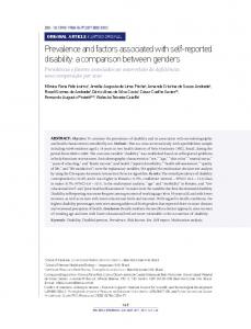
that for kurtosis and C6 statistics, the Theiler surrogate method rejects the null hypothesis at 100%. It is worth emphasing here that in [P. E. Rapp et al., 2001] the authors used the correlation dimension as the test statistic. For control time series that are iid normal, the Theiler surrogate method yields size rates that are zero in all three cases (skewness, kurtosis and C6 ), whereas for the bootstrap simulations the size rates are below the expected 5% level (see Tables 2 and 3). When the control time-series are iid uniform the size rates reported for the Theiler surrogate jumped from zero (skewness) to almost 100% (kurtosis and C6 ). This confirms to the expectation that Theiler’s surrogate is tuned for testing the linear normal null hypothesis if the test statistics is judiciously chosen. Note, however, that the surrogate method is rejecting linearity even though the control time series is purely linear. When the exponential distribution is considered, the Theiler method rejects the null hypothesis in all the cases. This seems to indicate that the Theiler method has more power when the distribution has a fat tail; if it is not taken into account that the method is again rejecting the linear null hypothesis. As for the bootstrap method, the size rates tend to increase with the complexity of the test statistics. This condition is somehow alleviated when the number of data points is increased. As stated before in the text, the normality of the distribution of the Q statistics was assumed. In order to check if such an assumption corresponds to reality, a simple test of normality was applied. In this test the Q statistics were plotted against the probabilities. The plot will be linear if the Q statistics are normally distributed. Figure 1 shows the results. The left panel are the normal plots for the bootstrap data (skewness, kurtosis and C6 ) whereas the right panel shows the same plots for the surrogate data. It is worth noticing that the bootstrap data deviates from the normality more than the surrogate counterpart. Therefore the use of the assumption of normality for bootstrap data is not without problems. 2.2. Confidence Intervals
It is often important to compute confidence intervals of an estimate of interest. For example, the 95% confidence interval of an estimate θˆ of a parameter θ is an interval I = [a, b] for which there is a prob-
M. J. Hinich, E. Mendes and L. Stone: A comparison between Standard Bootstrap and Skewness
Skewness
0.999 0.997 0.99 0.98 0.95 0.90 Probability
Probability
0.999 0.997 0.99 0.98 0.95 0.90 0.75 0.50 0.25
0.75 0.50 0.25 0.10 0.05 0.02 0.01 0.003 0.001
0.10 0.05 0.02 0.01 0.003 0.001 −0.2 −0.15 −0.1 −0.05
0 0.05 Data
0.1
0.15
−8
0.2
−6
−4
(a)
−2
2
4
6
8 −3
x 10
Skewness
0.999 0.997 0.99 0.98 0.95 0.90 Probability
0.999 0.997 0.99 0.98 0.95 0.90 Probability
0 Data
(b)
Skewness
0.75 0.50 0.25
0.75 0.50 0.25 0.10 0.05 0.02 0.01 0.003 0.001
0.10 0.05 0.02 0.01 0.003 0.001 −0.1
−0.05
0 Data
0.05
−8
0.1
−6
−4
(c)
−2
0 Data
2
4
6
8 −3
x 10
(d) Skewness
Skewness
0.999 0.997 0.99 0.98 0.95 0.90 Probability
0.999 0.997 0.99 0.98 0.95 0.90 Probability
7
0.75 0.50 0.25
0.75 0.50 0.25 0.10 0.05 0.02 0.01 0.003 0.001
0.10 0.05 0.02 0.01 0.003 0.001 1.6
1.8
2
2.2
(e)
2.4 Data
2.6
2.8
3
3.2
−10
−5
0 Data
5 −3
x 10
(f)
Figure 1: Skewness - normal plots: (a) Bootstrap - normal, (b) Surrogate - normal, (c) Bootstrap - uniform, (d) Surrogate uniform, (e) Bootstrap - exponential, (f) Surrogate - exponential
M. J. Hinich, E. Mendes and L. Stone: A comparison between Standard Bootstrap and
8
ability p = 0.95 that the true value of θ is in I. We check whether the bootstrap methods are capable of constructing confidence intervals that conform to those expected under the null hypothesis. When the variable of interest is the variance σ2 (but the method is similar in principle for other statistics) the confidence interval test is: 1. Construct M replications time-series using surrogate data or shuffle or bootstrap. 2. Compute sample quantiles of the M variances σˆ 2i of the M replications. 3. Calculate the 95% confidence interval [σˆ 2a , σˆ 2b ] for which 2.5% of the surrogates have a variance value less than σˆ 2a while 2.5% of the replications have a variance value greater than σˆ 2b . 4. Repeat steps 2., 3. & 4. for each replication to obtain confidence intervals. 5. Determine the ‘capture rates’ i.e., the proportion of cases for which σ2c =1 falls within these confidence intervals. Under the null hypothesis, for 95% confidence intervals, the capture rates are also expected to be close to 95%. Tables 4 and 5, for N=128 and N=2000 respectively, make clear that the capture rates computed for Theiler’s surrogate method are incorrect even for the case of normal data. The capture rate is markedly high for all test statistics, 100%, instead of 95% indicating that Theiler’s method produces too wide confidence intervals. It is worth pointing out that the capture rates for the surrogate method is either 0 or 100% in all cases which is far from the expected value of 95%.
Nor Uni Exp
Variance Theiler * * *
Shuf. * * *
Boot 93.53% 94.65% 87.89%
Skewness Theiler Shuf. 100% * 100% * 0% *
Boot 93.64% 95.02% 67.85%
Kurtosis Theiler 100% 0% 0%
Shuf. * * *
Boot 86.25% 96.97% 53.37%
C6 Theiler 100% 0% 0%
Shuf. * * *
Boot 96.71% 97.83% 24.50%
Table 4: Capture Rates for 95% confidence intervals (S=10,000; M=500; N=128). The “control” time series are taken to be normal (Nor) , uniform (Uni) or exponential (Exp) distributions. All the numerical values shown in the table are percentages. The ‘*’ indicates that the test fails due to lack of variability in the surrogates.
Nor Uni Exp
Variance Theiler * * *
Shuf. * * *
Boot 94.88% 94.91% 94.55%
Skewness Theiler Shuf. 100% * 100% * 0% *
Boot 94.77% 95.04% 87.36%
Kurtosis Theiler 100% 0% 0%
Shuf. * * *
Boot 93.16% 95.06% 79.93%
C6 Theiler 100% 0% 0%
Shuf. * * *
Boot 93.74% 95.25% 54.73%
Table 5: Capture Rates for 95% confidence intervals (S=10,000; M=500; N=2000). The “control” time series are taken to be normal (Nor) , uniform (Uni) or exponential (Exp) distributions. All the numerical values shown in the table are percentages. The ‘*’ indicates that the test fails due to lack of variability in the surrogates.
The shuffle method preserves all standardized cumulants and therefore cannot be used to verify the confidence intervals. On the other hand, the bootstrap method has capture rates close to the specified value q of 95% specially when the number of data points is set to 2000, but not within the tolerance of 0.05∗0.95 10,000 = 0.0022 as required. The worse cenario is for the exponentially distributed process, where
M. J. Hinich, E. Mendes and L. Stone: A comparison between Standard Bootstrap and
9
the capture reaches 54.73% when the sixth order standardized cumulant is used. This seems to indicate that care should be taken when dealing with fat tail distributions. According to Tables 2, 3, 4 and 5, the capture and size rates of all surrogate methods are unsatisfactory indicating that they should be used with caution. Recent work suggests that variants of the above bootstrap methods are reasonably successful; the results will be reported elsewhere.
3. The validity of the Surrogate Method - Discussion To further investigate the use of the surrogate method, two nonlinear models were considered: y(t) = −0.72026 y(t − 1)y(t − 1)y(t − 1)y(t − 1)y(t − 1) +0.20632×101 y(t − 1) −0.7107×10⁻² y(t − 1)y(t − 1)y(t − 1)y(t − 1) +0.20982×10⁻² −0.28051×10⁻⁴ y(t − 1)y(t − 1)y(t − 1) −0.55358×10⁻⁷ y(t − 1)y(t − 1)
(3)
y(t) = −0.10109×101 y(t − 1)y(t − 1) −0.71503 y(t − 1) +0.10109×101 +0.3 y(t − 2)
(4)
and
Equation (3) is a simple modification of the quintic logistic equation, y(t) = λy(t − 1)(1 − y4 (t − 1)) (where λ is a given parameter), whereas equation (4) is the Henon map counterpart, y(t) = 1 − 1.4y2 (t − 1) + 0.3y(t − 2). The objetive was to obtain two different nonlinear models from which data could be generated with mean equals zero and variance equals one. The skewness of data generated from modified quintic equation (3) is zero, therefore such an equation mimics a normal process up to the third order standardized cumulant. Figure 2 shows the first return maps for equations (3) and (4). Given the results presented in the previous section it is expected that the surrogate method will fail to reject the null hypothesis specially when the estimation of the skewness is considered. However the aim of this section is not to reproduce the results previously shown but to demonstrate that the hypothesis testing with the surrogate method is not well defined. To this end the following procedure was adopted: 1. Generate raw data from equations (3) and (4), and also nonlinear normal data. Here a static cubic function was used. 2. Generate surrogate data for each one of the data sets of 1. 3. Plot quantile-quantile plot for each raw and surrogate data Figures 3 and 4 show the quantile-quantile plots for both raw and surrogate data, respectively. From figure 3, it can be readily noticed that there is no agreement, that is, each different data set was drawn from different parent distributions. However, when the surrogate data for each one of the aforementioned processes are compared using the quantile-quantile plot, they seem to come from the same underlying parent density distribution (Figure 4). In fact, they are as the surrogate is approximately normal by
M. J. Hinich, E. Mendes and L. Stone: A comparison between Standard Bootstrap and 1.5
1
x(t −1)
0.5
0
−0.5
−1
−1.5 −1.5
−1
−0.5
0
0.5
1
1.5
x(t )
(a) 1.5 1 0.5 0 x(t −1)
−0.5 −1
−1.5 −2 −2.5 −2.5
−2
−1.5
−1
−0.5
0
0.5
1
1.5
x(t )
(b) Figure 2: First Return Maps for a) equation (3) and b) equation (4)
10
M. J. Hinich, E. Mendes and L. Stone: A comparison between Standard Bootstrap and Raw Data
Raw Data 20
1
15
0.5
10 Nonlinear Gaussian
1.5
Henon
0 −0.5 −1
5 0 −5
−1.5
−10
−2
−15
−2.5 −1.5
−1
−0.5
11
0 Logistic
0.5
1
1.5
(a)
−20 −1.5
−1
−0.5
0 Logistic
0.5
1
1.5
(b)
Raw Data 20 15
Nonlinear Gaussian
10 5 0 −5 −10 −15 −20 −2.5
−2
−1.5
−1
−0.5 Henon
0
0.5
1
1.5
(c) Figure 3: Quantile-Quantile plot: (a) Raw Data - Logistic X Henon, (b) Raw Data - Logistic X Nonlinear normal, (c) Raw Data - Henon X Nonlinear normal
Central Limit Theorem regardless of the shape of the parent density distribution. The surrogate method can therefore lead to spurious results for linearity since it requires absolute normality. In lay terms, how can one be sure that the rejection is based upon the linearity factor or simply because the data are not normal? Figure 5 shows that all surrogate data generated as described come from the same underlying distribution, that is, the normal distribution and therefore one can not distinguish between them.
4. Conclusions We have shown that the Theiler surrogate method is worthless as a time series bootstrap except for the restrictive linear and normal null hypothesis. Confidence intervals have been calculated for the surrogate
M. J. Hinich, E. Mendes and L. Stone: A comparison between Standard Bootstrap and Surrogate
Surrogate 5
4
4
3
3
2
2
Nonlinear Gaussian
5
Henon
1 0 −1 −2
1 0 −1 −2
−3
−3
−4
−4
−5 −5
0 Logistic
12
5
(a)
−5 −5
0 Logistic
5
(b)
Surrogate 5 4
Nonlinear Gaussian
3 2 1 0 −1 −2 −3 −4 −5 −5
0 Henon
5
(c) Figure 4: Quantile-Quantile plot: (a) Surrogate - Logistic X Henon, (b) Surrogate - Logistic X Nonlinear normal, (c) Surrogate - Henon X Nonlinear normal
and bootstrap methods. It has been shown that the surrogate method exhibits either 100% or 0% as capture rates even for the case when the control time series is a normal process. For exponentially and uniform distributed processes, the capture rates are even worse indicating that the surrogate method cannot be used for estimation of confidence intervals. Although the results for the Efron bootstrap are much better in comparison to the those ones for the surrogate data, it also fails to estimate confidence intervals within the required threshold. This is specially true for the higher standardized cumulants. A study on the drawbacks and possible solutions to the Theiler method surrogate has been recently published in [T. Schreiber and A. Schmitz, 2000], but they do not point up the critical issue of the normal null hypothesis.
M. J. Hinich, E. Mendes and L. Stone: A comparison between Standard Bootstrap and Surrogate
5
5
4
4
3
3
2
2
1
1
Gaussian
Gaussian
Surrogate
0 −1
0 −1
−2
−2
−3
−3
−4
−4
−5 −5
13
0 Logistic
5
(a)
−5 −5
0 Henon
5
(b)
Surrogate 5 4 3
Gaussian
2 1 0 −1 −2 −3 −4 −4
−3
−2
−1 0 1 Nonlinear Gaussian
2
3
4
(c) Figure 5: Quantile-Quantile plot: (a) Surrogate Logistic X normal, (b) Surrogate Henon X normal and c) Surrogate Nonlinean normal X normal
References W. Barnett, A. R. Gallant, M. J. Hinich, J. A. Jungeilges, D. T. Kaplan, and M. J. Jensen. A single–blind controlled competition among tests for nonlinearity and chaos. Journal of Econometrics, 82:157–192, 1997. J. Theiler and D. Prichard. Constrained-realization Monte_carlo method for Hypothesis Testing. Physica D, 94:221–235, 1996. B. Efron. Computers and the theory of statistics. SIAM Rev., 21:460–480, 1979a. B. Efron. Bootstrap Methods: Another Look at the Jacknife. Annals of Statistics, 7:1–26, 1979b.
M. J. Hinich, E. Mendes and L. Stone: A comparison between Standard Bootstrap and
14
B. Efron and R. Tibshirani. Bootstrap Methods for Standard Errors, Confidence Intervals, and Other Measures of Statistical Accuracy. Statist. Sci., 1(1):54–75, 1986. B. Efron and R. Tibshirani. Introduction to the Bootstrap. Chapman & Hall, Inc., 1993. J. Theiler, S. Eubank, A. Longtin, B. Galdrikian, and J.D. Farmer. Testing for nonlineaity in time series: the method of surrogate data. Physica D, 85:77, 1992. David R. Brillinger. Time Series Data Analysis and Theory. Holt, Rinehart and Winston, Inc., New York, 1975. D. Prichard and J. Theiler. Generating Surrogate Data for Time Series with Several Simultaneously measured variables. Phys. Rev. Lett, 73:991–954, 1994. D. Pierson and F. Moss. Detecting Periodic Unstable Points in Noisy Chaotic and Limite Cycle attractors with Applications to Biology. Phys. Rev. Lett, 75:2124–2127, 1995. T. Schreiber and A. Schmitz. Discrimination Power of Measures for Nonlinearity in a Time Series. Phys. Rev., 55:5443–5447, 1997. H. Kantz and T. Schreiber. Nonlinear time series analysis. Cambridge University Press, Cambridg, UK, 1997. T. Schreiber. Constrained Randomization of Time Series. Phys. Rev. Lett, 80:2105–2108, 1998. T. Schreiber and A. Schmitz. Surrogate Time Series (review paper). Physica D, 142:346–382, 2000. P. So, E. Ott, S. J. Schiff, D. T. Kaplan, T. Sauer, and C. Grebogi. Detecting Unstbale Periodic Orbits in Chaotic Experimental Data. Phys. Rev. Lett, 76:4705–4708, 1996. T. Chang, T. Sauer, and S.J. Schiff. Tests for Nonlinearity in Short Stationary Time Series. Chaos, 5: 118–126, 1995. Ying-Jie Lee, Yi-Sheng Zhu, Yu-Hong Xu, Min-Fen Shen, Hong-Xuan Zhang, and N. V. Thakor. Detection of Non-linearity in the EEG of Schizophrenic Patients. Clinical Neurophysiology, 112:1288– 1294, 2001. S.J. Schiff, K. Jerger, T. Chang, T. Sauer, and P.G. Aitken. Stochastic versus Deterministic Variability in Simple Neuronal Circuits II: Hippocampal Slice. Biophysical Journal, 67:684–691, 1994. M. C. Casdagli. Characterizing Nonlinearity in Weather and Epilepsy Data: A Personal View. Fields Institute Communications, 11:201–222, 1997. R. K. Pearson. Exploring process data. Journal of Process Control, 11:179–194, 2001. A. Mackay. Dictionary of Scientific Quotations. Institute of Physics Publishing, 1991. V. Clancy. Statistical methods in chemical analysis. Nature, 4036:339–340, 1947.
M. J. Hinich, E. Mendes and L. Stone: A comparison between Standard Bootstrap and
15
A. C. Davidson and D. V. Hinkley. Bootstrap Methods and Their Application. Cambridge University Press, 1997. Kung-Sik Chan. On the Validity of the Method of Surrogate Data. Fields Institute Communications, 11: 77–97, 1997. P. E. Rapp, C. J. Cellucci, and T. A. A. Watanabe. Surrogate Data Pathologies and the False-Positive Rejection of the Null Hypothesis. International Journal of Bifurcation and Chaos, 11(4):983–997, 2001.