There is a great need today for fast and reliable three dimensional scanning and model building in many different industrial, medical and robotic applications.
A Comparison of 3D Registration Algorithms for Autonomous Underground Mining Vehicles Martin Magnusson and Tom Duckett ¨ AASS, Orebro University Sweden Abstract. The ICP algorithm and its derivatives is the de facto standard for registration of 3D range-finder scans today. This paper presents a quantitative comparison between ICP and 3D NDT, a novel approach based on the normal distributions transform. The new method addresses two of the main problems of ICP: the fact that it does not make use of the local surface shape and the computationally demanding nearest-neighbour search. The results show that 3D NDT produces accurate results much faster, though it is more sensitive to error in the initial pose estimate.
1
Introduction
There is a great need today for fast and reliable three dimensional scanning and model building in many different industrial, medical and robotic applications. The main application considered in this paper is mine tunnel profiling and mapping. This is necessary to ensure that new tunnels have the desired shape, to measure the volume of material removed, to survey old tunnels and ensure that they are still safe, and, last but not least, to enable autonomous control of drill rigs and other mining vehicles. Scan matching can also be used for localisation — recognising a location within a previously built model of the world from a scan of the current surroundings. For this application, a laser range finder will be mounted on a drill rig commonly used for tunnel excavation (see figure 1). Several problems arise from this configuration. Naturally, it is only possible to see a very limited part of the mine at a time, and furthermore there is also a lot of self-occlusion from the vehicle itself. No matter where on the rig the sensor is placed, the drill booms and other parts of the rig will always be in the line of sight between the sensor and the walls. Therefore it is crucial to have reliable scan registration. Additionally, the environment is often wet or dusty. Airborne dust and wet, specular surfaces can lead to quite noisy sensor readings. The novel laser scanner used for our experiments is made by Optab Optronikinnovation AB. It is based on an infra-red laser, mounted in a housing that can be rotated around two axes, potentially making full
Fig. 1. An Atlas Copco drill rig in its natural environment.
Fig. 2. Four registered scans from the Kvarntorp mine (the tunnel data set), with different colours for clarity.
spherical scans. It has a range of approximately three to 45 metres, and both the latitudinal and longitudinal resolutions can be adjusted continuously to manage the trade-off between resolution and scanning speed. We have used an early prototype of the scanner, since it is not yet in production.
2
Registration
Three-dimensional pair-wise registration is the problem of matching two overlapping scans to build a consistent model, thus extrapolating the relative pose of one set with respect to the other. Given two scans and an initial guess for a transformation that will bring one set (the source) to the correct pose in the coordinate system of the other set (the target), the output is a refined transformation. In contrast to global surface matching algorithms, the class of registration algorithms search locally in pose space. Consequently, they may find an incorrect transformation if not given a good enough initial guess of the relative pose of the scans. This start pose can be selected manually, or in the case of a mobile robot, can be determined from odometry data. When matching high-resolution scans, one usually needs to choose a subset of points to compare. This can be done using a uniform or random subsampling. If topology data in the form of mesh faces or surface normals at the points are available, it is also possible to subsample in a more selective manner, such as choosing points where the normal gradient is high, or in a number of other ways. The preferred strategy for choosing points varies with the general shape of the surfaces. Surfaces that are generally flat and feature-less, such as long corridors, are notoriously difficult, but choosing samples so that the distribution of normals is as large as possible [1] forces the algorithm to pick more samples from the features that do exist (incisions, crevices and the like), and increases the chance of finding a correct match. 2.1
ICP
The iterative closest point (ICP) algorithm is widely used today for registration of 3D point clouds and polygonal meshes. ICP iteratively updates and refines the relative pose by minimising the sum of squared distances between corresponding points in the two scans, and was introduced in [2]. Since its conception, a large number of variants have been developed, and a good survey of different variations of ICP is presented in [1]. Once a set of points has been chosen, the algorithm proceeds to finding corresponding points in the
other scan. This search is where most of the execution time is spent. The naive way to do this is to pick for each point its closest neighbour by Euclidean distance. While this will not in general be the correct corresponding point, especially if the scans are far apart from each other, successive iterations will still usually converge to a good solution. To speed up the nearest-neighbour search, the points in the target data set are commonly stored in a kd-tree. If there are n points in the target data, and one wants to find the nearest neighbours of k points, the time needed for the search grows as O(n2/3 + k) for 3D data, plus the O(n log n) time needed for building the tree structure. Not all pairs that are found actually correspond to points that are close on the target surface. One may want to assign different weights to different point pairs, marking the confidence one has that they do indeed match. This can be done, for example, by setting the weight inversely proportional to the pointto-point distance and have lower weights for points further apart. For tunnel or corridor data, we have found that linear weighting can degrade performance. Because most points along the walls and ceiling will generally be well-aligned, their influence will overwhelm point pairs with larger distances, which correspond to corners and other features that are important. When registering scans with different amount of occlusions, taken from the same position, linear weighting is preferable. Some pairs will also need to be rejected entirely, to eliminate outlier points. This can be done using some heuristic to reject pairs where the points are far apart. Points lying on mesh boundaries should always be rejected. Otherwise, points from non-overlapping sections of the data may cause a systematic “drag” bias — see figure 3. Since it is difficult to determine the boundary points for point cloud data, we suggest using a decreasing distance threshold for rejection instead. This way, pairs that are separated by a large distance are used in early iterations to bring the scans closer, but in later iterations pairs where the points are far from each other are likely to be a non-overlapping point matched to a boundary point, and are rejected. Finally, the measured distances between the point pairs are minimised and the process is repeated again, with a new selection of points, until the algorithm has converged. There is a closed form solution for determining the transformation that minimises the total point-to-point error, which is described in [2]. The two largest problems with ICP are that firstly, it is a point-based method that does not consider the local shape of the surface around each point; and secondly, that the frequent nearest neighbour searches
resulting translation optimal translation
non-overlapping points
where qi and Ci are the average and covariance for the cell that contains point x. Since optimisation problems are generally formulated as minimisation problems, the score function is defined so that good parameters yield a large negative number. The rotation and translation parameters can be encoded in a vector p. Given a set of points xi and the transformation function T (p, x) to transform a point in space, the score function s(p) is defined as
overlapping points
Fig. 3. When the two scans do not overlap completely, allowing point pairs on the boundaries can introduce a systematic bias to the alignment process. are computationally expensive. Recent work [3] indicates that ICP alone is not suitable for mine mapping, although it has been used as the first step in a system that incorporates a subsequent global consistency adjustment [4]. 2.2
NDT
The normal distributions transform method for registration of 2D data was introduced in [5]. The key element in this algorithm is a new representation for the target point cloud. Instead of matching the source point cloud to the points in the target directly, the probability of measuring a point at a certain position is modelled by a linear combination of normal distributions. This gives a piecewise smooth representation of the target data, with continuous first and second order derivatives. Using this representation, it is possible to apply standard numerical optimisation methods for registration. The first step of the algorithm is to subdivide the space occupied by the target scan into regularly sized cells (cubes, in the 3D case). Then, for each cell bi that contains more than some minimum number of points, the average position qi of the points in the cell and the covariance matrix Ci (also known as the dispersion matrix) are calculated as qi =
1X xj , n j
(1)
Ci =
1 X (xj − qi )(xj − qi )T , n−1 j
(2)
where xj=1,...,n are the points contained in the cell. The probability that there is a point at position x in cell bi can then be modelled by the normal distribution N (q, C). The probability density function (PDF) is formulated as ¶ µ (x − qi )T C−1 i (x − qi ) , (3) p(x) = exp − 2
s(p) = −
X
p(T (p, xi )),
(4)
i
that is, the negated sum of probabilities that the transformed points of the source scan are actually lying on the target surface. Given the vector of transformation parameters p, Newton’s algorithm can be used to iteratively solve the equation H∆p = −g, where H and g are the Hessian and gradient of s. The increment ∆p is then added to the current estimate of the parameters in each iteration, so that p ← p + ∆p. For brevity, let q ≡ T (p, xi ) − qi . The entries for the gradient of the score function can be written as δs δq gi = = qT C−1 exp δpi δpi
µ
−qT C−1 q 2
¶ .
(5)
The entries of the Hessian are δs = δpi δpj ³ −qT C−1 q ´µ³ δq ´³ T −1 δq ´ exp qT C−1 −q C + 2 δpi δpj ¶ 2 δq T −1 δq T −1 δ q q C + C . (6) δpi δpj δpj δpi Hij =
The first-order and second-order partial deriva2 δq q tives δp and δpδi δp in the previous equations depend i j on the transformation function. In 2D, rotation is represented with a single value for the angle of rotation around the origin. General rotation in 3D is more complex. A robust 3D rotation representation requires both an axis and an angle. This leads to a 7-dimensional optimisation problem (three for the translation, three for the rotation axis, and one for the rotation angle), with quite expensive expressions for the partial derivatives. This paper presents a general 3D transformation function, and its partial derivatives with respect to the individual transformation parameters, as well as a quantitative comparison of 3D NDT with ICP. The trans-
Fig. 4. The source scan from the junction data set. formation function is T7 (x) = trx2 + c trx ry + srz trx rz − sry tx trx ry − srz try2 + c try rz + srx x + ty , tz trx rz + sry try rz − srx trz2 + c (7) where r = [rx ry rz ]T is the axis of rotation, s = sin φ, c = cos φ, t = 1 − cos φ, and φ is the rotation angle. Its derivatives with respect to the transformation parameters in p can be found in the Jacobian δq and Hessian matrices (8) and (9), where δp is the i 2
q i-th column of J and Hij = δpδi δp j However, if only small angles are considered, the rotation representation can be simplified substantially by using so-called Euler angles. Then rotations are represented as the product of three rotation matrices with angles φx , φy , and φz , rotating the point around the principal coordinate axes. Using Euler angles as a representation of general rotation has a number of defects: they are not always unique, and under certain conditions, they can lead to a situation called gimbal lock, where one degree of freedom is lost. See [6] for an exhaustive reference on rotations. For small 2 φ, sin φ ≈ φ and cos φ ≈ 1 − φ2 . Also, φ2 ≈ 0, and most terms of the derivatives reduce to zero. This improves the running time of the algorithm, at the cost of lower stability when registering scans with a large initial error.
3
Results
ICP and NDT were compared on two different data sets, both of which are scans from the underground test mine at Kvarntorp in Sweden. The junction
data set consists of two scans with different resolutions from the same position at the end of one tunnel, including a small passage to a neighbouring tunnel (see figure 4). The source scan has 139 642 points and the target scan has 72 417 points. These scans have obvious large-scale features, such as the end face of the tunnel and the passage. The tunnel data sets are scanned approximately 8 m apart in a section further down the tunnel, and contain 27 109 and 27 873 points, respectively. These two scans are depicted with two more consecutive scans in figure 2. The tunnel is around 12 m wide in both sets. For the junction data, the ground truth pose is simply zero translation and rotation, since the scans are taken from the same position and orientation. For the tunnel sets, the ground truth was determined manually by visual inspection of the aligned scans. Therefore the acceptable deviations from this estimated “ground truth” are larger than for the junction data. For these data sets, it is relatively easy to find the correct rotation, but the algorithms fail more often to converge to the correct translation. In order to make a quantitative comparison of the accuracy, the spatial and angular mismatch are measured separately. For the translation, the error is simply the Euclidean distance between the ground truth position and the estimated position. Measuring the rotational error is slightly more complicated. It is measured like this: if the difference in rotation is specified with the unit vector r and the angle φ, then er (r, φ) = kφrk is a scalar representation of that difference. Note that the elements of the 3D vector φr are not Euler angles, but the projections of the rotation axis onto the axes of the coordinate system. The times reported for ICP all include the creation time for a kd-tree used to speed up the nearestneighbour search. This only needs to be done once for each data set as long as it is not transformed. For a mapping application, where scans are matched in succession to the last one, these numbers are a good indication of the true time needed, but for an object recognition task where several models are registered to one fixed environment, it would be more fair to count only the registration time. The time needed to create the kd-tree for the target scan is approximately 4.4 s for the junction set, and 1.3 s for the tunnel set. A similar condition applies to NDT, where the equivalent to the kd-tree construction is the calculation of the means and covariances for the various PDFs, although this process is much faster than building a kd-tree. The box plots in the following figures all show the results of 50 runs. The median value is indicated by the thick black bar. The ends of the box show the first and third quartiles. The “whiskers” are then
T 1 0 0 0 1 0 0 0 1 x1 try + x3 s x1 trz − x2 s J = t(2x1 rx + x2 ry + x3 rz ) x2 trx − x3 s t(x1 rx + 2x2 ry + x3 rz ) x1 s + x2 trz x2 s + x3 trx −x1 s + x3 try t(x1 rx + x2 ry + 2x3 rz ) sA + cB sC + cD sE + cF
(8)
A = x1 rx2 − x1 + x2 rx ry + x3 rx rz , B = x2 rz − x3 ry , C = x1 rx ry + x2 ry2 − x2 + x3 ry rz , D = −x1 rz + x3 rx , E = x1 rx rz + x2 ry rz + x3 rz2 − x3 , F = x1 ry − x2 rx 00000 0 0 0 0 0 0 0 0 0 0 H= 0 0 0 a b 0 0 0 b e 0 0 0 c f 000dg
00 0 0 0 0 c d f g h i i j
2x1 srx + x2 sry + x3 srz x3 t x2 t 2x1 t , x1 sry + x3 c a = 0 , b = x1 t , c = 0 , d = 0 0 x t x1 srz − x2 c 1 x2 srx − x3 c 0 0 e = 2x2 t , f = x3 t , g = x1 srx + 2x2 sry + x3 srz , x t −x1 c + x2 srz 0 2 0 x2 c + x3 srx cA − sB , j = cC − sD −x1 c + x3 sry h = 0 ,i = 2x3 t x1 srx + x2 sry + 2x3 srz cE − sF
drawn towards the minimum and maximum values, but the maximum length is 1.5 times the interquartile range. Any values beyond the ends of the whiskers are considered outliers, and drawn as individual points. This method is the one commonly accepted among statisticians for drawing box plots. The initial estimate for each run was taken from the ground truth plus randomly generated error vectors — et for the translation, and er for the rotation — with different orientations for each run, but fixed magnitudes. All instances of ICP used uniformly random subsampling, nearest-neighbour correspondences, constant weights, and a maximum of 50 iterations. For junction, a fixed rejection threshold of 1 m was used, and for tunnel a decreasing threshold from 1 to 0 m. The results shown here did not use accelerated ICP as described in [2] and [7], as that caused the algorithm to “overshoot” in some cases. NDT uses axis/angle rotations and a cell size of 1 m. All the experiments were run on a Dell Latitude D800 with a 1600 MHz CPU and 512 MB of RAM. As can be seen from figures 5 and 6, NDT is substantially faster than ICP, and gives highly accurate results in most cases, although it fails in some cases when the initial error is large (as in figure 6). If a coarser sampling is used, or the target scan is also subsampled, it is possible to get running times comparable to those of NDT from ICP, but doing so also reduces the accuracy proportionally. For small disturbances, as in figure 5, the rotation error was negligible in all cases, and is therefore not shown here.
(9)
NDT ICP 0,00
0,01
0,02
0,03
0,04
Translation error (m)
0,05
0,06
0,07
NDT ICP 0
5
10
Time (s)
15
20
Fig. 5. Registration errors and running times for junction with errors ket k = 1 and ker k = 0.1. Figure 7 shows results from registering the tunnel scans. The median results here are still better than those of ICP, but it is not quite as reliable. We hypothesise that this is because of the smoothing effect of the PDFs. Features smaller than the side length of the cells are hidden because only the mean and covariance of the points within each cell are stored. The large scale features (walls and ceiling) of these scans are not generally enough to give an accurate registration. ICP can do a slightly better job of “sliding” two scans along the direction of the tunnel to make the small scale features (bumps on the walls) match.
4
Conclusions
The drag bias problem when non-overlapping points match to border points is elegantly solved with NDT. Non-overlapping points are simply disregarded since they fall into empty cells. This fact also illustrates a
NDT ICP 0,0
0,2
0,4
0,6
Translation error (m)
0,8
1,0
NDT ICP 0,00
0,10
0,20
0,30
Rotation error
0,40
0,50
0,60
NDT ICP 0
5
10
15
Time (s)
20
Fig. 6. Results for the same setup as in fig. 5, but with larger errors in the initial estimate. Here, ket k = 1 and ker k = 0.4. Rotation errors below 0.05 are good. NDT ICP 0,00
0,20
0,40
0,60
0,80
Translation error (m)
help when registering scans with weak features, just as it can for ICP, but this was not tested in the experiments covered by this paper. One can argue that NDT inherently includes a basic noise filter, since scattered sparse points do not count towards the PDF. However, only a few outlier points within a bin where most points are coplanar will disrupt the covariance so that the distribution is more spherical than planar. To conclude, the main advantage of ICP is that it can potentially make better use of small-scale features. It is also well-known, and is quite easy to to extend if sensor data with colour or other modalities is available. NDT, on the other hand, is much faster, and can produce results that are as accurate or better than those of ICP. However, NDT introduces another parameter, namely the size of the individual cells, and is more sensitive to error in the initial pose estimate.
1,00
5
Future work
NDT ICP 0,00
0,05
0,10
0,15
0,20
2
3
4
Rotation error
NDT ICP 0
1
Time (s)
Fig. 7. Results for registering tunnel with ket k = 0.5 and ker k = 0.1. weakness of NDT. As the chosen cell size gets smaller, so does the robustness with respect to the error in the initial pose estimate. If one scan is offset too much, it will not be able to “find” the other. Choosing too large cells, on the other hand, will hide smaller details, also leading to decreased accuracy. Also, the number of cells grows as O(l−3 ) with the side length l of the cells, so with small cells and voluminous data it will be necessary to use a sparse data structure for the cell grid. To make ICP’s nearest neighbour search efficient, it is usually necessary to put a threshold on the distance within which to search for corresponding points. This has a similar influence on the region of convergence as the finite cell size of NDT. It is possible to increase the region of convergence for NDT without sacrificing details by using a linear weighting of neighbouring cells if one is willing to trade off some speed. For example, the PDFs of the eight closest cells can be added with a weight based on the distance between the centre of the cell and the point in question. It is possible that normal based sampling would
The major difficulty when using NDT is how to choose a cell size that is large enough to give convergence, but small enough to be able to represent all important features. An interesting direction to explore would be adaptive and non-cubic cells, having smaller cells where needed, and larger cells for uniform regions. Different weighting schemes for NDT have not been pursued here. Possible options include smaller weights for cells with few points, or smaller weights for cells where the PDF is nearly spherical.
References 1. S. M. Rusinkiewicz, “Efficient variants of the ICP algorithm,” in The Third International Conference on 3D Digital Imaging and Modeling, 2001. 2. P. J. Besl and N. D. McKay, “A method for registration of 3-D shapes,” IEEE Transactions on Pattern Analysis and Machine Intelligence, vol. 14, Feb. 1992. 3. D. Ferguson, “Volumetric mapping with 3D registration,” tech. rep., Robotics Institute, Carnegie Mellon University, Nov. 2002. 4. S. Thrun, D. H¨ ahnel, D. Ferguson, M. Montemerlo, R. Triebel, W. Burgard, C. Baker, Z. Omohundro, S. Thayer, and W. Whittaker, “A system for volumetric robotic mapping of underground mines,” in Proc. ICRA, 2003. 5. P. Biber and W. Straßer, “The normal distributions transform: A new approach to laser scan matching,” in Proc. IROS, 2003. 6. S. L. Altmann, Rotations, Quaternions, and Double Groups. 1986. 7. D. A. Simon, Fast and Accurate Shape-Based Registration. PhD thesis, Carnegie Mellon University, 1996.