1D hydraulic models, a particle model with entrainment, and SAMOS, an .... 4. 203. â20. 14. 70. 48. 5. 23. â20. 16. 40. 38. 6. 38. 38. 15. 75. 31. 7. 48. â20. 15. 30.
A comparison of avalanche models with data from dry-snow avalanches at Ryggfonn, Norway D. Issler, C. B. Harbitz, K. Kristensen, K. Lied & A. S. Moe Norwegian Geotechnical Institute, P.O. Box 3930 Ullevål Stadion, N–0806 Oslo, Norway
M. Barbolini Univ. of Pavia, Hydraulics and Environmental Engineering Dept., Via Ferrata 1, I–27100 Pavia, Italy
F. V. De Blasio Inst. for Geosciences, University of Oslo, P.O. Box 1047 Blindern, N–0316 Oslo, Norway and International Centre for Geohazards, c/o NGI, P.O. Box 3930 Ullevål Stadion, N–0806 Oslo, Norway
G. Khazaradze Univ. of Barcelona, Dept. of Geodynamics and Geophysics, c/ Martí i Franquès s/n, E–08028 Barcelona, Spain
J. N. McElwaine Dept. of Applied Mathematics and Theoretical Physics, Centre for Mathematical Sciences, Cambridge University, Wilberforce Road, Cambridge, CB3 0WA, UK
A. I. Mears 555 County Road 16, Gunnison, Colorado 81230, USA
M. Naaim CEMAGREF, Division ETNA, 2 rue de la Papeterie, F–38402 St–Martin–d’Hères, France
R. Sailer Austrian Institute for Avalanche and Torrent Research, Hofburg, Rennweg 1, A–6020 Innsbruck, Austria ABSTRACT: Twelve well-documented dry-snow avalanches from the instrumented Ryggfonn path in western Norway were selected for back-calculations with several dynamical avalanche models. In each case, the run-out distance, the front velocity in the lower track, the extent of the deposits and the depth profile along a line are known. A 16 m high and 100 m wide retention dam in the run-out zone is often overflowed by avalanches but retains a considerable fraction of their mass. The tested models comprise a quasi-analytic block model, two 1D hydraulic models, a particle model with entrainment, and SAMOS, an advanced 2D/3D two-layer model. For each model, a wide range of friction parameters was needed to reproduce the twelve events, and none of the models matches the deposit distributions of all avalanches with fair accuracy. Explicit representation of the intermediate-density layer in dry-snow avalanches and accurate numerical schemes are expected to improve the modelling of dam interactions. 1 INTRODUCTION As a geotechnical material, snow has striking similarities with other soil types, especially clay, but also several decisive differences. Compared to landslides, snow avalanches are a very frequent phenomenon, yet the return period of extreme avalanches is beyond individual memory and the traces of avalanches are not as clearly preserved as e.g. debris-flow deposits. Protection of settlements by means of landuse planning therefore usually requires extrapolation from a short observation period to return periods of several hundred years. Technical measures like catching and deflecting dams are sometimes cost-effective protection schemes but dimensioning them optimally also depends on sound knowledge of the dynamical properties of extreme avalanches. A multitude of dy-
namical avalanche models have been developed over the past 50 years (Harbitz 1998) and measurements on full-size avalanches and laboratory flows carried out for 40 years. With many open questions still remaining in avalanche dynamics, current work aims at a deeper understanding of the basic avalanche processes through detailed measurements in the field and the laboratory, and at improving models on this basis. Among other things, the latter should be capable of realistically simulating the interaction with dams. As part of co-ordinated efforts at the European level, NGI operates a full-scale instrumented test site in the Ryggfonn avalanche path in western Norway, which features a 16 m high and 100 m wide catching dam in the run-out zone. In order to assess the capabilities and limitations of existing models in a re1
alistic context, we selected twelve well-documented dry-snow avalanches from the 1983–2000 Ryggfonn data and five avalanche models that are currently in use for hazard mapping and represent different levels of complexity. For each of the models and each of the twelve avalanches, we determined the optimum friction parameters for simulating the measured run-out distance and velocity. The same initial conditions and parameters were then used to obtain the model predictions for the run-out distance and deposit geometry if there were no dam. Obviously, we do not know Nature’s “true” answer, but the differences in the impact behaviour of the five models are clearly highlighted.
and f = 5/4 in NIS. Many models, like VARA1D, assume the depth-averaged longitudinal stress per unit density to be hydrostatic, σ˜ s = −(h/2)g cos φ. Various formulations have been proposed for the bed shear stress τb . In VARA-1D, the usual Coulomb dryfriction term is accompanied by a drag term proportional to the velocity squared; note that it is not proportional to the flow depth, in contrast to the FSB model (1): τ˜b = sgn(u)(µgh cos φ + ku 2 ), 5 · 10−3
where k ∼ is an adjustable parameter. The NIS model recognizes the granular nature of avalanches and represents the bed-normal stress as the sum of effective and dispersive stresses; it is assumed that the latter is proportional to the square of the shear rate. Besides the Coulomb friction proportional to the effective normal stress (including centrifugal effects), there is also a dispersive contribution to the shear stress. In practical applications, only a restricted implementation of the full NIS model is used; the bottom shear stress then reduces to (Lied et al. 2004, pages 33–37)) � �α � � 2 τ˜b = sgn(v) µgh cos φ + 2 + κµh u 2 , (5) h and the longitudinal normal stress is not hydrostatic: h σ˜ s = (1 − (tan φ − µ)α1 ) g cos φ. (6) 2 Typical parameter values are µ ∼ 0.3, m ∼ α2 ∼ 10−3 m2 and α1 ∼ 10. The PLK model (Perla et al. 1984) describes avalanches as collections of snow blocks, each of which obeys the equation of motion � � v2 dv ± bv. (7) = g sin φ − sgn(v) µg cos φ + dt 3 The last term, with the sign chosen stochastically, represents interaction of a block with its neighbours, b being a measure of the collision frequency. A userdetermined number of particles per unit length is added to the system as the front advances. An (ad hoc) assumption important in connection with dam impacts is that, at concave slope changes, the original momentum component normal to the new slope is lost. SAMOS (Sampl & Zwinger 2004) combines a 2D depth-averaged dense-flow model with a 3D powder-snow avalanche model. The dense part of the flow is a Lagrangean implementation of the Savage– Hutter model (Savage & Hutter 1991) at low velocities; above a threshold determined by the dispersive stresses a drag term replaces the dry-friction term. Snow entrainment and the effect of path curvature on dry friction are taken into account. In contrast to the other models, a digital terrain model was used in the simulations.
2 MAIN FEATURES OF THE MODELS The earliest avalanche models described the motion of a point of mass M on a slope z(x) according to Newton’s equation Ma = Mg sin φ − F f , where a = dv/dt is the acceleration along the slope, g the gravitational acceleration, φ the local slope angle and F f the friction force, which needs to be specified in terms of M, g, v and φ. A simple extension is the Flexible Sliding Block (FSB) model that considers an avalanche as a perfectly flexible slab of fixed length l. Its centre of mass obeys formally the same equation of motion, but φ, F f (and the curvature κ, see below) are to be considered means over the path segment presently occupied by the avalanche. The FSB model includes dry friction proportional to the apparent weight (taking into account centrifugal forces) and “turbulent” friction or drag: � � � v2 � 2 F f = sgn(v)M µ · g cos φ + κv + . (1) 3 The drag term is assumed proportional to the avalanche mass and 3 = O(103 m) is the length scale over which the kinetic energy decays due to drag. The solution of the equation of motion can be expressed in terms of quadratures. One-dimensional hydraulic models like VARA-1D (Natale et al. 1994) and NIS (Norem et al. 1989) are the most frequently used in practical applications today. The depth-integrated mass and momentum balance equations have the structure ∂h ∂(hu) + = we , ∂t ∂s
(2)
∂(hu) ∂( f hu 2 ) ∂(h σ˜ s ) + = gh sin φ + − τ˜b . ∂t ∂s ∂s
(3)
(4)
where s is the distance along the curved path, h is the flow height, u the depth-averaged velocity, we the snow-entrainment rate per unit density (neglected in most models). The Boussinesq coefficient f depends on the velocity profile; f = 1 in VARA-1D 2
Table 1: Ryggfonn avalanches used in the numerical simulations. The over-run length is measured from the downstream base of the dam, with estimated values for the thick deposits in parentheses. The avalanche volume refers to the estimated release volume. No.
Overrun (m) all core
Freebd. (m)
Volume (103 m3 )
Velocity (m s−1 )
1 2 3 4 5 6 7 8 9 10 11 12
148 −22 48 203 23 38 48 151 29 58 173 311
14 13 16 14 16 15 15 6 16 15 5 5
100 45 20 70 40 75 30 20 40 20 100 80
46 23 34 48 38 31 43 35 33 35 45 49
Altitude [m a.s.l.]
700
Figure 1: Overview map of the Ryggfonn avalanche path with the dam and deposit area of the avalanche event 3. The co-ordinates at the left and bottom sides are in meters, north is towards the top of the figure.
3
? −22 ? −20 −20 38 −20 ? −5 ? 70 150
Terrain Avalanche deposit, to scale Deposit exaggerated 5 times
680 660 640 620 600 1500
1550
1600 1650 1700 1750 1800 Horizontal distance from release area [m]
1850
1900
Figure 2: Deposit profile of the avalanche event 12 drawn to scale (shaded) and five times exaggerated (dashed line).
THE RYGGFONN AVALANCHES
Located near Stryn in western Norway at an altitude from 1500 to 600 m a.s.l, the Ryggfonn fullscale avalanche test site (Figure 1) has been in operation since 1980. Avalanches starting in the bowlshaped release zone are channelled in the track before they begin to spread laterally on an alluvial fan and impact on a 100 m wide and 16 m high catching dam in the run-out zone after a horizontal travelling distance of approximately 1600 m. The deposit volume of observed avalanches ranges from 10,000 m3 to 500,000 m3 , the maximum velocities reach up to 60 m s−1 . From the avalanche arrival times at two pressure-measurement locations 320 and 230 m upstream from the dam, the front velocity can be determined, albeit with some uncertainty because sensors of different sensitivity were used prior to 2002. For the present study, we selected twelve dry-snow avalanches for which surveys providing estimates of the release area, fracture depth, runout length, deposit area and volume had been carried out (Table 1). All the selected avalanches hit the dam, and either were stopped by it or over-topped it. The snow density in the release area was extrapolated from NGI’s snow measurement station at Fonnbu, located a few kilometers away at an elevation of 920 m a. s. l. The initial conditions for the simulations are thus known with reasonable accuracy. Some of the avalanches occurred after earlier
avalanches had partially filled up the retention volume upstream of the dam. On the one hand, this made it easier for the next avalanche to overtop the dam, but on the other hand the friction on the old deposit may have been significantly increased. Table 1 records the freeboard for each event, i.e. the vertical distance between the snow surface at the dam foot and the top of the dam. With release volumes from 20,000 m3 to 100,000 m3 and front velocities from 23 m s−1 to 49 m s−1 , the selected avalanches span a wide range of sizes. Important information about the behaviour of a model at the dam is contained in the deposit distribution. For each of the twelve avalanches, the deposit depth was measured along a line crossing the dam, and the edges of the deposits were mapped (Figures 1 and 2); all maps and profiles are presented in (Lied et al. 2004, pages 25–98). Many of the profiles show deep deposits (up to 18 m) only to a certain point—most often the dam—and a rather abrupt decrease to 2 m or even much less just downstream from that point. This deposit structure may indicate the presence of two different flow regimes in these avalanches, namely a dense, relatively slow core preceded by a dilute, fluidised layer moving at much higher speed (Schaerer & Salway 1980; Schaer & Issler 2001). (The deposits from the suspension layer were not mapped.) The deep deposits of avalanches 3
Table 2: Optimum parameter values for simulating the twelve Ryggfonn avalanches. The drag terms were transformed to a canonical form with a dimensionless coefficient k by dividing by appropriate powers of the release height. The much higher k-value for SAMOS reflects the fact that this model switches between dry friction and “turbulent” drag according to the local dispersive pressure. No.
FSB µ
103 k
PLK µ
103 k
VARA-1D µ 103 k
NIS µ
103 k
SAMOS µ 103 k
1 2 3 4 5 6 7 8 9 10 11 12
0.35 0.26 0.35 0.25 0.49 0.32 0.51 0.20 0.38 0.34 0.28 0.06
1.7 6.1 2.6 1.9 0.5 3.6 0.1 3.1 2.4 2.4 1.8 3.1
0.25 0.25 0.20 0.30 0.30 0.25 0.30 0.25 0.25 0.25 0.25 0.25
1.9 4.1 3.0 3.6 2.8 3.2 3.2 2.4 3.0 3.5 2.4 1.0
0.39 0.17 0.41 0.20 0.41 0.42 0.41 0.28 0.41 0.42 0.28 0.10
0.2 2.3 0.3 0.5 0.3 0.3 0.3 0.5 0.1 0.2 0.5 0.6
0.40 0.39 0.28 0.25 0.33 0.42 0.42 0.24 0.32 0.38 0.32 0.18
1.5 3.3 3.4 1.3 2.1 2.8 0.8 3.0 2.5 2.2 1.6 2.0
0.34 0.49 0.36 0.29 0.42 0.45 0.45 0.27 0.40 0.36 0.36 0.19
22 22 22 22 22 22 22 22 22 22 22 22
Average Standard deviation
0.32 0.12
2.4 1.5
0.26 0.03
2.8 0.8
0.33 0.12
0.5 0.6
0.33 0.08
2.2 0.8
0.37 0.09
22 0
friction parameters for matching the observed run-out distance and front velocity. With these values, the runout distance on a modified path profile with the freeboard of the dam removed was calculated. The details of the simulation procedure varied somewhat between models due to differences in their input requirements and resource needs. For the quasi-analytic FSB model, the dry-friction coefficient µ was obtained in terms of the dimensionless drag coefficient k for each avalanche. One thousand simulations per avalanche were performed with VARA-1D. With NIS, the parameter space was scanned as well, but with fewer simulations. In the PLK runs, the parameters were optimised starting from their values used in practical hazard mapping. SAMOS requires very substantial computational resources so that only a few simulations could be carried out for each avalanche; the internal friction angle and the dynamic friction coefficient were kept fixed at φ = 35◦ and k = 0.022, respectively, and only the base friction angle δ = arctan µ was varied. The SAMOS simulations represent mixed dense-flow/powder-snow avalanches, but only the dense part was considered for velocities, runout distances and parameter optimisation. In order to allow (semi-quantitative) comparison of the optimum parameters between models (Table 2), the drag terms were transformed to have the same structure, with a non-dimensional drag coefficient k, by scaling them with the appropriate power of the release depth. The parameter sets that best reproduce the observed events at Ryggfonn are much less pessimistic than the parameters recommended for predicting extreme avalanches in Switzerland using a model quite similar to VARA-1D (Bartelt et al. 1999). We cannot conclusively explain this discrepancy but
11 and 12 extend to the river and to the foot of the opposite slope, respectively. The corresponding overrun lengths are about 70 m instead of 173 m and 150 m instead of 311 m, respectively. Present-day models do not distinguish these flow regimes, therefore the runout distance of the fluidised layer was used in calibrating the models in this study. Reanalysis of pressure data from Ryggfonn indicates that the density in the head of dry-snow avalanches tends to be below 100 kg m−3 and that the velocity decays steadily after passage of the head while the density increases (P. Gauer, pers. comm.). The mapped outlines of the avalanches presented in (Lied et al. 2004) show that the lateral spreading of the avalanche debris around the dam differs considerably between events. This is not very surprising because it is expected to depend on a number of highly variable factors like the location and width of the release area, the flow velocity, the snow properties and earlier deposits. Among the compared models, only the 2D code SAMOS is in principle able to take these effects into account. No simple relation between speed, volume, runout and spread-out ratio has been found so far. As an example, avalanche 1 with a volume of 100,000 m3 , velocity 46 m s−1 and over-run length of 148 m showed almost no spread whereas avalanche 11, which had about the same volume, over-run length and velocity, doubled its width over the last 150 m. The extreme case is avalanche 4, whose width increased nearly four-fold. 4
SIMULATION RESULTS
For each of the five models and each of the twelve avalanches, we determined the best combination of 4
Table 3: Observed and simulated deposit distributions: Estimated percentage of mass stopped above the downstream foot of the dam. For each model the numbers in the right column refer to simulations with the same model parameters, but without a dam. No. 1 2 3 4 5 6 7 8 9 10 11 12
Meas. (%)
FSB (%) (%)
VARA-1D (%) (%)
NIS (%)
(%)
PLK (%) (%)
SAMOS (%) (%)
67 100 87 79 91 87 90 64 94 75 65 38
0 100 55 0 80 65 9 0 74 45 0 0
23 100 70 16 85 70 64 27 75 54 8 11
16 100 44 0 95 72 34 0 94 36 0 0
11 83 30 0 90 62 31 0 89 28 0 0
57 100 9 65 100 61 93 16 95 97 14 11
20 100 70 14 99 85 90 26 92 88 38 4
0 62 39 0 56 46 0 0 55 30 0 0
6 95 53 9 76 60 56 21 60 38 4 9
5 10 9 11 7 5 9 8 8 7 7 11
16 95 50 11 86 84 84 18 67 68 25 3
Table 4: Shortening of simulated run-out distances due to the presence of the dam. For each event and model, the same parameters were used as in the corresponding optimized simulation with the dam.
note that (i) except for the largest avalanches in our sample, the return periods are less than five years, and (ii) the dissipative effect of the dam is underestimated in these models (except by PLK), so higher friction values along the entire path must be used to compensate for this deficiency. Except for the very highly fluidised avalanche 12, the observed run-out distances could generally be matched fairly well by all models. Significant discrepancies occurred for the front velocity, with deviations as large as 10 m s−1 in some cases. Unfortunately, the front velocity data are not precise enough to blame only the models for the discrepancies. The average dry-friction coefficient over all twelve avalanches was close to 0.32 with a standard deviation between 0.08 and 0.12 for most models. In the case of the calibration of the PLK model, the parameters were chosen as close as possible to those found in extensive consulting experience. This fact explains the somewhat lower value of µ together with an elevated value of k as well as the smaller range of both these parameters in the PLK model. (This choice reflects itself also in a poorer match of the velocity compared to the other models.) It is likely that the parameter range of the other models could also be reduced if similar preferences were imposed during calibration. From Table 3 it is apparent that most simulations underestimated the retention ratio, i.e. the fraction of avalanche mass stopped upstream of the downstream foot of the dam, even though the run-out distance and the velocity in the lower track were tuned to the measured values. About 30 % of the simulations gave a mass distribution close to the observed one, in 10 % of the cases the retention ratio was overestimated, and it was too small in about 60 %. For six of the twelve avalanches, at most one estimate was correct, all others being too low. The only readily recognizable trend in the discrepancies between model results and obser-
No.
Freebd. (m)
FSB (m)
VARA-1D (m)
NIS (m)
PLK (m)
SAMOS (m)
1 2 3 4 5 6 7 8 9 10 11 12
14 13 16 5 16 14 14 5 16 15 5 5
−2 63 16 −4 24 19 11 −15 19 14 −6 −5
0 15 10 0 40 20 15 0 15 10 0 0
39 57 40 59 1 28 36 36 4 39 44 36
222 129 171 13 71 136 88 46 164 106 34 36
30 25 15 55 105 5 40 15 20 35 0 0
11
10
35
101
29
Avg.
vations is that FSB, VARA-1D and NIS generally predict too low retention ratios while PLK and SAMOS overestimate them in certain cases. Underestimation of the retention ratio by FSB and NIS may be linked to an underestimation of the longitudinal spreading of the avalanche—since the run-out distance was forced to agree with observations, the deposits were concentrated too far downstream. After the optimum parameters had been determined for each combination of avalanche event and model, the same parameter set was applied with the same initial conditions, but on a terrain profile from which the freeboard of the dam had been removed (Tables 3 and 4). The “correct” run-out shortening due to the dam is not known, of course, but the tables highlight how differently the models react to a large object in the path. The energy dissipation due to Coulomb friction is 5
ACKNOWLEDGEMENTS
insensitive to the dam (if the avalanche is fast enough to overtop the dam); also, the drag effects do not differ much with or without the dam. Accordingly, VARA1D predicts a mere 10 m of run-out shortening on average. The PLK model exhibits very pronounced run-out shortening with about 100 m on average: The ad hoc prescription for momentum reduction in concave bends reduces the kinetic energy to roughly one quarter of its value before the dam. A more physical approach is to account for the centrifugal effects in bends (FSB, NIS, SAMOS); friction increases in the concave bends at the foot of the dam and decreases it in convex ones at the crown, but to a lesser degree because the velocity is smaller there. The net extra dissipation of energy per unit mass at the dam is (Lied et al. 2004, page 50) 1E ≈ −4µg H α = O(−g H ), (8) ◦ where the deflection angle α is about 40 and H ≤ 16 m at Ryggfonn. With µ ∼ 0.4, this translates into a run-out shortening of about 40 m in the case of full freeboard. This estimate is reasonably well confirmed by the NIS and SAMOS, but not the FSB calculations.
This work was funded by the European Union 5th Framework Programme through the project SATSIE (EU Contract no. EVG1–CT2002–00059) and by the Norwegian Geotechnical Institute. REFERENCES Bartelt, P., Salm, B. & Gruber, U. (1999). Calculating dense snow avalanche runout using a Voellmyfluid model with active/passive longitudinal straining. J. Glaciol. 45(150): 242–254. Gray, J. M. N. T., Tai, Y.-C. & Noelle, S. (2003). Shock waves, dead-zones and particle-free regions in rapid granular free surface flows. J. Fluid Mech. 491: 161– 181. Hákonardóttir, K. M., Hogg, A. J., Jóhannessson, T. & Tómasson, G. G. (2003). A laboratory study of the retarding effects of braking mounds on snow avalanches. J. Glaciol. 49(165): 191–200. Harbitz, C. (1998). A survey of computational models for snow avalanche motion. NGI Report 581220–1. Oslo, Norway: SAME Collaboration / Norwegian Geotechnical Institute. Lied, K., Moe, A., Kristensen, K. & Issler, D. (2004). Ryggfonn. Full scale avalanche test site and the effect of the catching dam. In M. Naaim and F. Naaim-Bouvet (eds), Snow and avalanches test sites. Proc. Intl. Seminar on Snow and Avalanches Test Sites in the Memory of Philippe Revol, Grenoble 22–23 November 2001: 25–98. Antony, France: Cemagref Editions. Natale, L., Nettuno, L. & Savi, F. (1994). Numerical simulation of snow dense avalanche: an hydraulic approach. In M. H. Hamza (ed.), Proc. 24th Intl. Conf. on Modeling and Simulations, 2–4 May 1994, Pittsburgh, Pennsylvania: 233–236. Anaheim, California: IASTED. Norem, H., Irgens, F. & Schieldrop, B. (1989). Simulation of snow-avalanche flow in run-out zones. Annals Glaciol. 13: 218–225. Perla, R., Lied, K. & Kristensen, K. (1984). Particle simulation of snow avalanche motion. Cold Regions Sci. Technol. 9: 191–202. Sampl, P. & Zwinger, T. (2004). Avalanche simulation with SAMOS. Annals Glaciol. 38: 393–398. Savage, S. B. & Hutter, K. (1991). The dynamics of avalanches of granular material from initiation to runout. Part I: Analysis. Acta Mechanica 86: 201–223. Schaer, M. & Issler, D. (2001). Particle densities, velocities, and size distributions in large avalanches from impact-sensor measurements. Annals Glaciol. 32: 321– 327. Schaerer, P. A. & Salway, A. A. (1980). Seismic and impact-pressure monitoring of flowing avalanches. J. Glaciol. 26(94): 179–187. Tai, Y. C., Noelle, S., Gray, J. M. N. T. & Hutter, K. (2002). Shock-capturing and front-tracking methods for granular avalanches. J. Comp. Phys. 175(1): 269–301.
5 CONCLUSIONS Several conclusions relevant to avalanche hazard mapping and future model development can be drawn from our restricted study. First, the range of friction and drag parameters needed to reproduce different avalanches in the same track is extremely wide. “Blind” application of models may lead to completely wrong results; automated generation of detailed hazard maps is inadmissible with present-day models. Second, future models should allow for flowregime changes in order to describe the fluidised layer observed in front of many if not all dry-snow avalanches. This may both improve the modelling of the pressure distribution in the run-out zone and narrow the range of friction parameters needed for reproducing observations. Third, the power of current personal computers allows very rapid 1D computations of avalanche flow; hence there is little need to further use block models like FSB. Even though 2D simulations are now also quite feasible on PCs, the effort required for input preparation for the time being still limits their application to situations where an avalanche may split in several branches or chose its path depending on the velocity. e.g. on alluvial fans or in bends of shallow channels. Finally, so-called conservative formulations of the balance equations should be combined with shockcapturing numerical schemes (Tai et al. 2002) to account for shocks that develop in the impact of granular flows on obstacles (Hákonardóttir et al. 2003). First results from such codes (Gray et al. 2003) appear very promising. 6