Dec 30, 2014 - denotes an i-th block of time series, then the block length begins from i. X for. Ni ..... High-frequency financial time series of returns is featured.
189
Croatian Operational Research Review CRORR 5(2014), 189–202
A comparison of four different block bootstrap methods Boris Radovanov1,∗ and Aleksandra Marcikić1 1
Faculty of Economics Subotica, University of Novi Sad Segedinski put 9-11, Serbia E-mail: 〈{radovanovb, amarcikic}@ef.uns.ac.rs〉
Abstract. The paper contains a description of four different block bootstrap methods, i.e., non-overlapping block bootstrap, overlapping block bootstrap (moving block bootstrap), stationary block bootstrap and subsampling. Furthermore, the basic goal of this paper is to quantify relative efficiency of each mentioned block bootstrap procedure and then to compare those methods. To achieve the goal, we measure mean square errors of estimation variance returns. The returns are calculated from 1250 daily observations of Serbian stock market index values BELEX15 from April 2009 to April 2014. Thereby, considering the effects of potential changes in decisions according to variations in the sample length and purposes of the use, this paper introduces stability analysis which contains robustness testing of the different sample size and the different block length. Testing results indicate some changes in bootstrap method efficiencies when altering the sample size or the block length. Key words: Block bootstrap, returns, stability analysis Received: September 29, 2014; accepted: December 2, 2014; available online: December 30, 2014
1. Introduction If one chooses an adequate bootstrap mechanism along with an appropriate sample, it could be plausible to achieve persuasive approximation of statistics of the whole population [8]. Every bootstrap procedure is derived from the original Efron’s bootstrap procedure [3], which was primarily assigned to independent and identically distributed data. Therefore, following the basic principles of the i.i.d. bootstrap, other types of procedures appear according to an increased number of statistical requirements. Although the created set of bootstrap procedures is successfully used in many applications, the comprehension of scientific society about bootstrap application power still remains unknown. Due to this fact and understanding the differences of empirical usability in particular scientific disciplines, the problem of acceptable bootstrap procedure selection remains opened. The ∗
Corresponding author.
http://www.hdoi.hr/crorr-journal
©2014 Croatian Operational Research Society
190
Boris Radovanov and Aleksandra Marcikić
selection understatement affects the opinion among many econometrics researchers that bootstrap procedure selection is not an easy task [10]. The paper encompasses four related sections. After the introduction, the second section of research provides a basic knowledge of the block bootstrap procedure and its four applied methodologies. The third section describes the comparison process of block bootstrap results derived from two topics: testing for dynamics in the conditional mean of variance returns and modeling volatility of returns. Finally, this paper ends by some recommendations as well as concluding remarks.
2. Block bootstrap In case of lack of experience in econometric model specification, the block bootstrap procedure is proposed as one of the most widely used bootstrap methods in a domain of time series. The main reason for defining such method is maintaining the time series dependency structure within a pseudo-sample. The block bootstrap is developed separately by Hall [5] and Carlstain [2] and Künsch [7]. They all started from the criteria of creating blocks of consecutive data. The procedure divides the original time series into blocks of individual observation units or estimated residuals, where the bootstrap data inside each block are created using the classical i.i.d. bootstrap. At the beginning of block bootstrap development, two possible tendencies of forming blocks, the nonoverlapping and the overlapping block bootstrap, appear.
2.1. Moving block bootstrap In separate research, Künsch [7] and Liu and Singh [9] have formulated a new scheme of creating pseudo-samples called the moving block bootstrap or the overlapping block bootstrap. Unlike the i.i.d. bootstrap process that forms new artificial samples by taking random observations from the initial sample, the moving block bootstrap performs the sampling procedure only within a row of formed blocks. As a result of such procedure, the time series structure of original data is preserved within each particular block of data. Also, the initial assumption is that the general block length will continue to increase with additional observations in the original sample. Based on random sample X 1 , X 2 ,..., X n , the procedure defines estimation by using the moving block bootstrap process of θˆ = T ( F ) , where F is an n
n
n
empirical function of random sample distribution. If one starts from the assumption that l ≡ ln ∈ [1, n] is an integer, the example for dependent data usually requests that l → ∞ and n −1l → 0 when n → ∞ . Anyway, a specific description of this method must start from the block length l constraint. If
A comparison of four different block bootstrap methods
191
Bi = ( X i ,..., X i + l −1 ) denotes an i-th block of time series, then the block length
begins from X i for 1 ≤ i ≤ N , where N = n − l + 1 is presented as the number of blocks within the bootstrap sample. In order to form a sample from the moving block bootstrap method it is necessary to choose randomly a certain number of blocks from the set {B1 ,..., BN }. Therefore, B1* ,..., Bk* represents a random sample with repetitions from the set {B1 ,..., BN }, where each block contains the same number of elements l. With respect to observations within block Bi* presented as (X (*i −1)l +1 ,..., X il* ) , where i = 1,..., k , bootstrap observations construct a sample X 1* ,..., X m* based on the moving block bootstrap with block size m ≡ kl . Thus the version of the moving block bootstrap for parameter θˆn is denoted as θ m* ,n and presented in the following form: θ m* , n = T (Fm*, n ) ,
(1)
where Fm*,n shows the empirical distribution of moving block bootstrap samples X 1* ,..., X m* . As resampled blocks of observations (X 1* ,..., X l* )′ , (X (*l +1) ,..., X 2*l )′ ,..., (X (*k −1)l +1 ,..., X kl* )′
are independent and identically distributed vectors with:
P* (( X 1* ,..., X l* )′ = ( X j ,..., X j + l −1 )′) = P* ( I j = j ) = N −1 ,
(2)
1 ≤ j ≤ N , where P* represents a conditional probability. According to l → ∞ with n, any finite-dimensional joint probability distribution can be revealed eventually from resampled observations. As a result, the moving block bootstrap is able to efficiently approximate features of the process within the whole population. Considered estimation θˆn = T ( Fn ) includes few common estimations that are not sufficient for application in terms of time series. The primary reason for such condition is that the estimation θˆn depends only on one-dimensional marginal empirical distribution Fn , and thus it does not cover standard statistics. Hence, it is necessary to observe a more general version of the moving block bootstrap which envelopes those statistics:
θˆn = T ( Fp ,n ) ,
(3)
where Fp , n is a p – dimensional empirical function, T (⋅) represents a subset of
all probability measures set ( X i ,..., X i + l −1 )∈ R p . A dimension p ≥ 1 is given as a constant in the form of an integer or p → ∞ with n.
192
Boris Radovanov and Aleksandra Marcikić
In contrast, this paper also recognizes a rule of forming blocks established by Carlstein [2]. For the simplicity of the procedure, one considers the estimation θˆn = T ( Fp ,n ) , where p = 1. The main feature of the mentioned block forming procedure is non-overlapping of data segments contained in the sequence of blocks. Therefore, this procedure is called the non-overlapping block bootstrap. If one begins, with the assumption that l ≡ ln ∈ [1, n] is an integer, then the number of blocks of observed time series b ≥ 1 is the largest integer that accomplishes the relation lb ≤ n . It allows forming of blocks as ′ Bi′ = (X (i −1)l +1 ,..., X il ) , i = 1,..., b . After forming a series of non-overlapped blocks within original time series, the procedure of bootstrap implementation is the ′
′
same as the one mentioned above. After random selection of blocks B1* ,..., Bk* with replacement from the set {B1′,..., Bb′ } , where m = kl , the empirical
′
distribution of bootstrap sample Fm*,n is formed. Thus the bootstrap version of estimation θˆn is given as:
′ ′ θ m* , n = T Fm*, n .
(4)
Although the definition of bootstrap estimation is very similar in both
′
mentioned bootstrap procedures, the resulting estimations θ m* ,n and θ m* ,n have different distribution properties. However, using a simple example for arithmetic mean E E* (θ m* , n ) − E* (θ m* , n′ ) = O(l / n 2 ) , the difference between these two bootstrap 2
techniques becomes negligible in case of a large sample [8]. Except for direct application to original data, some versions of block bootstrap procedures are adopted in processing series of residuals formed from the set of estimation models. In that case, there is no need to create the best suitable finite-dimensional model, but the emphasis is on resampling of estimated residuals using previously formed blocks. According to the process of block replacement, it is possible that some randomly selected block of residuals is not used in a pseudo-sample, while another one is used several times. If the blocks of residuals are long enough, the autocorrelation structure of estimated model errors should be accurately reflected through the bootstrap errors and with forming of a bootstrap sample it offers a chance to make an adequate distribution approximation of required statistics from the original data sample [4]. Using the small length of block l would adversely affect procedure performances.
A comparison of four different block bootstrap methods
193
2.2. Subsampling The usage of different data subsets in approximation of bias and variance measures for statistics of interest is a common practice in application of independent and identically distributed observations. However, the subseries of dependent observations could be useful in creating valid variance estimations, bias measures and distributions of samples under weak assumptions [2] [6]. In order to provide an appropriate explanation of the subsampling method, it is inevitable to indicate a few input assumptions. If θˆn = Tn ( X 1 , X 2 ,..., X n ) is an estimation of the parameter θ , with adequate normalization of the parameter an > 0 , the probability distribution Gn ( x) = P (an (θˆn − θ ) ≤ x weakly converges to the marginal distribution G (x) , or:
G n ( x) → G ( x) when n → ∞ .
(5)
For all continuous values x ∈ R . Let 1 ≤ l ≤ n be a given integer so that Bi = ( X i ,..., X i + l −1 ) for 1 ≤ i ≤ N in case of overlapping blocks. Then the estimation using subsampling Gn is given as:
Gˆ n ( x) = N −1
N
∑ I (a (θˆ l
i ,l
− θˆn ) ≤ x ,
(6)
i =1
where θˆi, l is a copy of the estimation θˆn from the block Bi = ( X i ,..., X i + l −1 ) defined as θˆi ,l = Tl ( Bi ) . It can be noticed that Tl (⋅) is a substitution for Tn (⋅) in order to estimate the statistics of subsample θˆ , considering the fact that the block Bi contains only l observations.
i, l
2.3. Stationary bootstrap Similarly to the block bootstrap, the stationary bootstrap, created by Politis and Romano [12], includes the resampling procedure of initial data in order to form new pseudo-samples of time series and reestimate statistics of interest, but with one significant difference related with time series stationarity. The stationary bootstrap is generally acceptable in application of weakly dependent stationary time series. In case of the block bootstrap, the new samples of time series are not stationary, so the involvement of the stationary bootstrap tries to remove this undesirable statistical characteristic. Therefore, according to the original data sample X 1 , X 2 ,..., X n , the pseudo time series X 1* , X 2* ,..., X n* is
194
Boris Radovanov and Aleksandra Marcikić
generated using an adequate scheme of creating new stationary samples. The defined procedure tries to mimic characteristics of the original sample by keeping a desirable feature of time series stationarity within pseudo time series samples. To achieve this, the bootstap time series occurs with resampling of different length blocks, where the length of each block is approximated by the geometric distribution. Starting from the assumption that the original sample X 1 , X 2 ,..., X n is a strictly stationary and weakly dependent time series, the distribution of statistics of interest Tn ( X ) = Tn ( X 1 , X 2 ,..., X n ) is estimated. Let Bil = ( X i ,..., X i + l −1 ) be the block which contains l repeatedly observations starting from X i . In order to ensure that all initial observations have the same drawing probability, the circular block scheme is suggested. Independently of X 1 , X 2 ,..., X n , let L1 , L2 ,... be the series of independent and identically distributed random variables with geometric distribution:
P ( Li = m) = (1 − p ) m −1 p ,
(7)
where p ∈ {0,1} and p → 0 , np → ∞ . Independently of X i and Li , let I1 , I 2 ,... be the sequence of independent and identically distributed variables with discrete uniform distribution from the set {1,..., n} . Hence, pseudo time series X 1* , X 2* ,..., X n* are generated by the sequence of random length blocks BI1 , L1 , BI 2 , L2 ,... . First L1 observations are determined using the first block BI1 , L1
of observation series X I1 ,..., X I1 + L1 −1 that are followed by the second L2 number of observations in the block BI 2 , L2 of series X I 2 ,..., X I 2 + L2 −1 . The defined process continues until it reaches n observations within the pseudo-sample, although it is clear that mentioned process leaves space to expand the pseudo-sample for an arbitrary number of observations. Other variants of the stationary bootstrap based on the pattern of forming random length blocks are also possible. Instead of the assumption of the geometric distribution for Li , and the discrete uniform distribution for I i , the bootstrap procedure considered other forms of data distribution. Considering the difficulty of bootstrap method application from the block length point of view, variance estimations using the stationary or the moving block bootstrap are similar to each other, since p −1 is approximately equal to l [12]. The stationary bootstrap is basically represented by the weighted average of distributions of standard error estimates generated by the moving block bootstrap. Therefore, the stationary bootstrap of variance estimates is less sensitive when selecting a probability p than the moving block bootstrap when selecting the block length l. This leads to the fact that the selection of probability p in the stationary
195
A comparison of four different block bootstrap methods
bootstrap is less important than the selection of the block length l in the moving block bootstrap.
3. Comparison of block bootstrap methods
MSE
The next chapter serves to create an appropriate ground for a practical comparison of the mentioned bootstrap methods. There remains an open question about quantification of relative efficiency of respective block bootstrap methods. Lahiri introduces an empirical example where the moving block bootstrap surpasses all other versions of block bootstrap methods according to criteria of the mean squared error [8]. After all, the same author asks whether a similar situation will happen if there is any variation in the sample size or the application point. If the performances are measured for each method with different optimal block length, the comparison problem appears the as well. Similarly, for the purpose of examining efficient application, Figure 1 illustrates a preliminary comparison of mean squared errors in estimation of the variance of BELEX15 returns using four most frequently used block bootstrap methods in the interval from April 2009 to April 2014, or 1,250 daily observations, whereby the number of repetitions is B = 1,000. 0.0005 0.00045 0.0004 0.00035 MBB
0.0003
NBB
0.00025
SBB
0.0002
SS
0.00015 0.0001 0.00005 0
1
2
3
4
5
6
7
8
9
10
11
12
13
14
15
l
Figure 1: Preliminary comparison of block bootstrap methods
Figure 1 presents mean squared errors of four block bootstrap methods (MBB – Moving block bootstrap, NBB – Non-overlapping block bootstrap, SBB – Stationary block bootstrap and SS-Subsampling). This figure shows the dominance of the moving block bootstrap with an application of the small block length. When the block length increases, the errors in all four bootstrap methods are slowly equalizing. Although the obtained results stand with a big question mark from the aspect of the variation in the sample size or the
196
Boris Radovanov and Aleksandra Marcikić
application area, this analysis, encouraged by similar research results of many authors, gives a certain assurance and motivates a further application of mentioned methods. From the theoretical point of view and according to the concept of the mean squared error, achieved stationarity using the stationary bootstrap does not contribute significantly to a decrease in estimation biases. Also, the usage of overlapping and non-overlapping blocks provides asymptotically the same degree of bias as long as the expected block length l is asymptotically equivalent. On the other hand, despite the differences in forming blocks, the methods have the same variance order of resulting estimations. This fact is interesting in case of the stationary bootstrap where an additional rate of stochastic in resampled blocks shows an asymptotic increase in variance comparing to the other block methods. The presented asymptotic approximation of this type serves as a benchmark for comparison of individual methods, especially in case of analysis of a different sample size and application area.
3.1. Testing for dynamics in the conditional mean of variance returns Tests of dynamic characteristics are considered to be some kind of analytical performance verification of bootstrap methods. Therefore, testing for dynamics of the conditional mean represents the initial step in successful analysis and prediction of the stock returns movement. Although a serious number of authors emphasizes the inability to predict returns in the short term, one can not ignore the importance of stock return tracking in the long term. Market participants often use a trending strategy, considering that by keeping the momentum of a growing trend they will have greater odds to achieve positive financial results. Related to lack of ability to efficiently predict trends in the following periods, market participants predominantly used appropriate methodology to track serial correlation of returns. Numerous studies have found that daily stock returns reveal a positive low-serial correlation that is frequently recognized to non-synchronous trading effects, i.e., the efficiency market hypothesis [13]. Consequently, a strong need for testing autoregressive dynamics in returns emerges. Ruiz and Pascual propose asymptotic standard errors and bootstrap p – values for testing and conclude that the results are similar [13]. If θˆ is an estimated parameter, θˆb* an appropriate estimation of the b-th bootstrap replication and θ * an average of θˆb* , then the standard error using the bootstrap is calculated by the following form:
A comparison of four different block bootstrap methods
s* (θˆ) =
1 B ˆ* (θ b − θ * ) 2 B − 1 b =1
197 (8)
∑
The standard error in equation (8) can be used in the same way as every other asymptotically valid standard error used to estimate confidence intervals or perform some test statistics [10]. The p – value presents the estimate of the marginal significance level, i.e., the probability of an event established by the null hypothesis. Through p – values it is possible to determine the empirical and the bootstrap distribution based on a certain data generating process. Therefore, the p – value is expressed by the binary indicator function presented in equation (9), in which the estimated and bootstrap values of variables are compared to original data as: pˆ * =
1 B
B
∑ I(X
* b
≤ X).
(9)
b =1
The indicator function takes value 1 if the claim is true or 0 otherwise. Equation (9) can also be presented as pˆ * = 1 − Fn* , where Fn* denotes the empirical distribution function from the bootstrap process, which alters the real distribution F0 .
To illustrate the effect of conditional dynamics on bootstrap densities, B = 1000 series have been bootstrapped by the following AR(1) – GARCH(1,1) model: X t = µ + φ1 X t −1 + ε t
σ t2 = α 0 + α1 ⋅ ε t2−1 + β ⋅ σ t2−1 where
,
(10)
X t represents the series of returns derived from stock prices X t = log( pt / pt −1 ) , σ t is the volatility and ε t is a white noise. Table 1 presents statistics of dynamics in variance returns for four different block bootstrap methods in two sample sizes, i.e., 750 daily observations and 1,250 daily observations. According to criteria of minimizing mean squared errors, the optimal block length is calculated in terms of statistics of interest and the sample size. At the first sight, Table 1 shows that all block bootstraps offer p – values closed to the original sample, i.e., all bootstrap techniques have density distributions of statistics of interest similar to the original data. Comparing standard errors and mean squared errors in the bootstrap and the empirical distribution indicates that the bootstrap procedures give better results. Also, changes in the sample size have less effect on bootstrap results
198
Boris Radovanov and Aleksandra Marcikić
than on empirical results. In other words, the bootstrap procedures perform more robust results. The analysis of bootstrap results shows the dominance of the moving block and the stationary block bootstrap in both samples. Bootstrap method Empirical Block Moving block Stationary block Subsampling
T
p-value
st.dev.
MSE
750 1250 750 1250 750 1250 750 1250 750 1250
0.51225 0.52456 0.52014 0.52414 0.52114 0.52874 0.52208 0.53042 0.52027 0.52509
0.01658 0.01549 0.01655 0.01548 0.01628 0.01516 0.01633 0.01517 0.01612 0.01449
0.000498 0.000452 0.000469 0.000427 0.000314 0.000284 0.000355 0.000406 0.000506 0.000471
Table 1: Testing the dynamics for conditional mean
3.2. Modeling volatility of returns Volatility of returns represents the uncertainty in stock price movements of risky assets in a certain period of time. Volatility represents one of the most important concepts in the domain of finance [1]. Volatility, measured by the standard deviation or the variance of returns, is often used as an initial measure of the total asset risk. High-frequency financial time series of returns is featured by a leptokurtic distribution and autocorrelation in consecutive observations [11]. This fact emphasizes that volatility has a significant impact on variance fluctuation, i.e., heteroskedasticity. Furthermore, the expected volatility has one of the most important roles in modern financial theory. Since the conditional volatility is a very important segment in dynamic risk management, the best characteristics in modeling and forecasting of the future volatility have been shown by the models that contain information about lagged return values. High-frequency financial data are usually explained by the presence of conditional heteroskedasticity [11]. Therefore, one of the leading methods in dynamic volatility modeling is the general autoregressive conditional heteroskedasticity model (GARCH).
199
A comparison of four different block bootstrap methods Bootstrap method Empirical
Block
Moving block
Stationary block
Subsampling
T 750 1250 750 1250 750 1250 750 1250 750 1250
α0 (t-test) 0.00001 (5.6934) 0.00001 (6.3959) 0.00001 (4.5022) 0.00000 (5.0155) 0.00001 (4.8772) 0.00001 (6.9091) 0.00001 (6.6722) 0.00001 (7.9817) 0.00001 (5.4804) 0.00001 (6.6091)
α1 (t-test) 0.23265 (7.1359) 0.18102 (8.7254) 0.24326 (6.8841) 0.20785 (8.1144) 0.24255 (7.3805) 0.20392 (9.5716) 0.20140 (6.1856) 0.15493 (8.1491) 0.19961 (7.8802) 0.20392 (9.5716)
β (t-test) 0.71765 (23.454) 0.78669 (41.684) 0.75024 (27.485) 0.78322 (41.289) 0.74632 (30.959) 0.77644 (48.576) 0.74168 (31.053) 0.81020 (53.904) 0.78546 (41.414) 0.77644 (48.576)
St.dev.
MSE
0.016420
0.000383
0.014951
0.000316
0.014221
0.000360
0.013101
0.000301
0.013956
0.000310
0.012593
0.000250
0.014470
0.000192
0.013755
0.000129
0.014217
0.000317
0.012676
0.000232
Table 2: Estimation of parameters in the GARCH model
Table 2 contains estimation of parameters in GARCH model specification. t – statistics of each parameter is presented in parenthese. Given results show that bootstrap methods are less sensitive to changes in the sample size. Estimated values from the original sample indicate the stationarity of the process in variance if α1 + β < 1 . Thus the stationarity of the estimated GARCH model denotes convergence of the conditional variance predicted values to the mean with a change in time horizon, while that convergence is not expected if α1 + β ≥ 1 . The aforementioned bootstrap methods mainly lead to reduction of estimation errors, i.e., increase in t – statistics compared to the initial sample. Besides, these methods are getting the sum of parameters α1 + β closer to 1 without compromising quality forecasting assumptions. Calculated standard deviations mostly decrease with the use of some versions of the block bootstrap compared to the original data set and thus explain further growth in stability of estimating GARCH model parameters. Furthermore, prediction performances within the sample show smaller mean squared errors in case of the moving block, the stationary block bootstrap and subsampling. GARCH model estimations made by the mentioned methods are getting closer to the integrated process and increase the convergence of predicted values to the mean in the long term.
200
Boris Radovanov and Aleksandra Marcikić
In terms of sample stability, this paper involves the measurement of parameter stability when changing the sample size. In order to keep basic features of the time series dynamic structure in and out of the sample by using the GARCH model, it is necessary to sustain parameter stability. Regarding this, the F – test is involved in variance analysis as follows:
∑ε − ∑ε 2 t
F* =
n2
∑ε
2′ t
2′ t
,
(11)
n1 − k
where
∑ε
sample,
2 t
∑ε
is the sum of squared residuals of the GARCH model using a longer 2′ t
is the sum of squared residuals of a smaller sample, k is the
number of estimated parameters, n1 is the number of observations in a smaller
sample and n2 is the difference in observations between two observed samples. Bootstrap method Empirical Block Moving block Stationary block Subsampling
F - test 0.4073 0.4098 0.3945 0.4022 0.3987
Table 3: Testing parameter stability
Table 3 shows the calculated results of F – statistics. These results are compared with a critical value and if F * < F (α , n2 , n1 − k ) , the conclusion is that there is no statistically significant difference between estimated parameters in both samples with a different size, i.e., parameter stability is satisfied. The critical value in this case is F (5%;500;747 ) = 0.87 with 5% of error. Thus, all F – statistics are below the critical value and indicate that there is statistically significant stability of estimated parameters. Nevertheless, there are no evident changes in the dynamic structure of volatility returns time series in case of BELEX15.
A comparison of four different block bootstrap methods
201
4. Conclusion Four different block bootstrap methods, i.e., non-overlapping block bootstrap, overlapping block bootstrap (moving block bootstrap), stationary block bootstrap and subsampling, were tested in this paper. Bootstrap methods could mostly give an approximation of the theoretical value with high accuracy. However, the conclusion does not imply that bootstrap methods can be used without any verification. Instead, bootstrap results are treated with caution. Consequently, every new situation caused by a certain financial problem and belonging statistics requires additional attention in order to obtain results that are closer to the actual distribution. Regarding this, the presented paper takes a closer look on each proposed bootstrap method and suggests the use of some of them in defined situations. In the case of testing the dynamic structure of time series, we propose the use of the moving block and the stationary block bootstrap, while in the case of modeling and forecasting volatility, each block bootstrap procedure except the block bootstrap gives reliable results. Overall, the moving block bootstrap procedure shows the lowest errors in estimation and prediction in and out of the sample. Finally, changing the block length affects overall results, but at the same time it does not make a different decision about the comparison among bootstrap relative performances.
References [1] Brooks, C. (2004). Introductory Econometrics for Finance. Cambridge: University Press. [2] Carlstein, E. (1986). The use of subseries values for estimating the variance of a general statistic from a stationary sequence. The Annals of Statistics, 14(3), 1171– 1179. [3] Efron, B. (1979). Bootstrap methods: Another look at the jackknife. Annals of Statistics, 7(1), 1–26. [4] Godfrey, L. (2009). Bootstrap Tests for Regression Models. Hampshire: Palgrave Texts in Econometrics. [5] Hall, P. (1985). Resampling a coverage pattern. Stochastic Process and Their Applications Journal, 20(2), 231–246. [6] Hall, P., Jing, B. (1996). On sample reuse methods for dependent data. Journal of Royal Statistical Society, 58(4), 727–737. [7] Künsch, H. (1989). The jackknife and the bootstrap for general stationary observations. Annals of Statistics, 17(3), 1217–1241. [8] Lahiri, S.N. (2003). Resampling Methods for Dependent Data. New York: Springer – Verlag. [9] Liu, R., Singh, K. (1992). Moving Blocks Jackknife and Bootstrap Capture Weak Dependance. New York: John Wiley & Sons.
202
Boris Radovanov and Aleksandra Marcikić
[10] MacKinnon, J. (2006). Bootstrap methods in econometrics. The Economic Record, 82, Special Issue, 2–18. [11] Pascual, L., Romo, J., Ruiz, E., (2000). Forecasting returns and volatilities in GARCH processes using the bootstrap. Available from: http://halweb.uc3m.es/esp/Personal/personas/romo/_papers/jbes.pdf [Accessed on 15 September 2014] [12] Politis, D., Romano, J. (1994). The stationary bootstrap. Journal of the American Statistical Association, 89(428), 1303–1313. [13] Ruiz, E., Pascual, L. (2002). Bootstrapping financial time series. Journal of Economic Surveys, 16(3), 271–300.