A Comparison of Multisensor Integration Methods for Land Cover Classification in the Brazilian Amazon Dengsheng Lu,1 Guiying Li, and Emilio Moran Anthropological Center for Training and Research on Global Environmental Change (ACT), Indiana University, Bloomington, Indiana 47405
Luciano Dutra
National Institute for Space Research, 12227-010 São Jose dos Campos, SP, Brazil
Mateus Batistella
Brazilian Agricultural Research Corporation, EMBRAPA Satellite Monitoring, 13070-115 Campinas, São Paulo, Brazil
Abstract: Many data fusion methods are available, but it is poorly understood which fusion method is suitable for integrating Landsat Thematic Mapper (TM) and radar data for land cover classification. This research explores the integration of Landsat TM and radar images (i.e., ALOS PALSAR L-band and RADARSAT-2 C-band) for land cover classification in a moist tropical region of the Brazilian Amazon. Different data fusion methods—principal component analysis (PCA), wavelet-merging technique (Wavelet), high-pass filter resolution-merging (HPF), and normalized multiplication (NMM)—were explored. Land cover classification was conducted with maximum likelihood classification based on different scenarios. This research indicates that individual radar data yield much poorer land cover classifications than TM data, and PALSAR L-band data perform relatively better than RADARSAT-2 C-band data. Compared to the TM data, the Wavelet multisensor fusion improved overall classification by 3.3%–5.7%, HPF performed similarly, but PCA and NMM reduced overall classification accuracy by 5.1%–6.1% and 7.6% –12.7%, respectively. Different polarization options, such as HH and HV, work similarly when used in data fusion. This research underscores the importance of selecting a suitable data fusion method that can preserve spectral fidelity while improving spatial resolution.
INTRODUCTION An increasing variety of remotely sensed data is becoming available, from very high spatial resolution images such as QuickBird and WorldView to very coarse spatial resolution data obtained from the MODerate resolution Imaging Spectroradiometer 1
Corresponding author; email:
[email protected]
345 GIScience & Remote Sensing, 2011, 48, No. 3, p. 345–370. DOI: 10.2747/1548-1603.48.3.345 Copyright © 2011 by Bellwether Publishing, Ltd. All rights reserved.
346
lu et al.
(MODIS) and the Advanced Very High Resolution Radiometer (AVHRR). Spectral resolution ranges from the limited number of multispectral bands of the Landsat Thematic Mapper (TM) to the over 200 bands of the hyperspectral Hyperion. Passive optical sensors such as Landsat and SPOT can be contrasted with active sensors such as the Advanced Land Observation Satellite (ALOS) Phased Array type L-band Synthetic Aperture Radar (PALSAR) and RADARSAT. Several researchers and scholars, such as Estes and Loveland (1999) and Lefsky and Cohen (2003), have previously reviewed the characteristics of major types of remote sensing data. Effective use of different kinds of remotely sensed data, such as the integration of optical and radar data, has become an active research topic because of the advantages of distinct features in data collection and representation. In general, the combination of multisensor data can be based on incorporation of one sensor’s data as extra bands added to multi spectral imagery or based on other data fusion methods (Haack and Herold, 2007; Lu et al., 2007). Data fusion is often used for the integration of multisensor or multiresolution data to enhance visual interpretation and/or to improve the performance of quantitative analysis (Klonus and Ehlers, 2007; Lu and Weng, 2007). In general, data fusion involves two major procedures: (1) geometric co-registration of two datasets; and (2) mixture of spectral and spatial information contents to generate a new dataset that contains the enhanced information from both originals (Lu and Weng, 2007). Accurate co-registration between two datasets is extremely important for precisely extracting information content from both datasets, especially for linear features such as roads and rivers. Radiometric and atmospheric calibration may also be required before multisensor data are merged. Data fusion can incorporate the same sensor data with different spatial resolutions, such as from QuickBird, IKONOS, SPOT, and Landsat ETM+ (Enhanced Thematic Mapper Plus), including multispectral and panchromatic data (Ehlers et al., 2010; Zhang, 2010). Data from different sensors may also be combined, such as from Landsat TM and radar or hyperspectral and lidar (LIght Detection And Ranging) (Lucas et al., 2006; Lu et al., 2007; Ali et al., 2009; McNairn et al., 2009). Many data fusion methods, such as principal component analysis (PCA), the wavelet-merging technique (Wavelet), intensity-hue-saturation (IHS), Brovey transform, color normalization spectral sharpening, Gram Schmidt fusion, support vector machine, and Ehlers fusion, have been developed to integrate spectral and spatial information (Gong, 1994; Pohl and van Genderen, 1998; Chen and Stow, 2003; Klonus and Ehlers, 2007; Dong et al., 2009; Ceamanos et al., 2010; Ehlers et al., 2010; Zhang, 2010). Data fusion can work on three levels—pixel, feature, and decision (Gong, 1994; Jimenez et al., 1999; Chitroub, 2010). Solberg et al. (1996) broadly divided data fusion methods into four categories: statistical, fuzzy logic, evidential reasoning, and neural network. Pohl and van Genderen (1998) reviewed data fusion methods, including color-related techniques, statistical/numerical methods, and various combinations of these methods. A recent review paper by Zhang (2010) further outlined multisource data fusion techniques and discussed their trends. A challenge in selecting a data fusion method is evaluating the fused results. Li et al. (2010) discussed the measures based on multivariate statistical analysis to evaluate the quality of data fusion results. An alternative is based on the comparison of land cover classification results from different data fusion methods (Lu et al., 2008).
multisensor integration methods
347
Fig. 1. Study area in and around Altamira, Pará State, Brazil.
Although many data fusion methods are available (e.g., Pohl and van Genderen, 1998; Zhang, 2010), it is not fully understood which fusion method is suitable for integrating Landsat TM and radar data to improve land cover classification, especially in moist tropical regions. It is also unclear which radar wavelength (e.g., L-band or C-band) and which polarization option (e.g., HH and HV) have better land cover classification performance for the same data fusion method. Therefore, this research aims to identify which wavelength and polarization and which data fusion method—PCA, Wavelet, high-pass filter resolution-merging method (HPF), or normalized multiplication method (NMM)—yield better classification in the moist tropical region. Landsat TM, ALOS PALSAR L-band HH and HV images, and RADARSAT-2 C-band HH and HV images were used for exploring the data fusion methods for improving land cover classification in Altamira, Pará State, Brazil. STUDY AREA The study area consists of the city of Altamira, located along the Transamazon Highway (BR-230) in the northern Brazilian state of Pará, as well as the surrounding area, encompassing a total of roughly 3,116 km2. The city lies on the Xingu River at the eastern edge of the study area (Fig. 1). Extensive deforestation in the region began
348
lu et al.
in the early 1970s, coincident with the construction of the Transamazon Highway (Moran, 1981), and has continued since that time. The dominant native types of vegetation are mature moist forest and liana forest. Deforestation has led to a complex landscape consisting of different stages of secondary succession, pasture, and agricultural lands (Moran et al., 1994; Moran and Brondizio, 1998). Various stages of successional vegetation are distributed along the Transamazon Highway and feeder roads. Annual rainfall in Altamira is approximately 2,000 mm and is concentrated from late October through early June; the dry period occurs between June and September. Average temperature is about 26° C. METHODS Field Data Collection and Determination of a Land Cover Classification System Sample plots for different land cover types, especially for different stages of secondary succession and pasture, were collected in the Altamira study area during July–August 2009. Prior to the field work, candidate sample locations of complex vegetation areas were identified in the laboratory. Primary forest is distributed away from the roads and different stages of succession vegetation, pastures, and agricultural lands are distributed along the main and secondary roads, forming the familiar “fishbone” pattern of deforestation. Because of the difficulty in accessing forested sites in moist tropical regions like this study area, random allocation of sample plots for field survey is not feasible. Therefore, the majority of sample plots relevant to non-forest vegetation and pastures were allocated along the roadsides. In each sample area, the locations of different vegetation cover types were recorded using a global positioning system (GPS) device, and detailed descriptions of vegetation stand structures (e.g., height, canopy cover, composition of dominant tree species) were recorded. Field photos also were taken of each vegetation type. Sketch map forms were used in conjunction with small field maps showing the candidate sample locations to note the spatial extents and patch shapes of vegetation cover types in the area surrounding the GPS point. The sample plots were used to create representative region of interest (ROI) polygons. Based on the field survey and a QuickBird image, a total of 432 plots were sampled. Of the sampled plots, 220 ROIs were used as training plots for image classification, and 212 ROIs were used as test plots for accuracy assessment. ROI polygons were created by identifying areas of uniform pixel reflectance in window sizes from approximately 3 × 3 pixels to 9 × 9 pixels on the Landsat TM imagery, depending on the patch sizes of different land covers. Based on the research objectives, compatibility with previous research work (Mausel et al., 1993; Moran et al., 1994; Moran and Brondizio, 1998), and field surveys, three forest classes (upland [UPF], flooding [FLF], and liana [LIF]), three succession stages (initial [SS1], intermediate [SS2], and advanced [SS3]), agropasture (AGP), and three non-vegetated classes (water [WAT], wetland [WET], and urban [URB]) were developed and used for the land cover classification system. Due to cloud conditions in the rainy season, good-quality optical sensor data are mainly available in the dry season (July and August in this study area). During the dry season, agricultural lands and pastures have similar spectral features and cannot be separated using optical sensor data; thus, they are grouped into the AGP class. An emphasis of this research was to explore improvement in extraction of vegetation, rather than non-vegetation categories.
multisensor integration methods
349
Table 1. Summary of Remotely Sensed Data Used in Research Sensor data
Major characteristics of: Different sensor data
Selected sensor data
Landsat 5 TM
Six spectral bands, covering visible, Path/row: 226/62; UTM zone: 22, near-infrared, and shortwave infra- south; image acquisition date: 2 July red bands with 30 × 30 m spatial 2008; sun elevation angle: 50.4°. resolution; one thermal band with 120 m spatial resolution.
ALOS PALSAR
Radar L-band HH and HV polarization options with 12.5 m pixel spacing.
RADARSAT-2
Radar C-band HH and HV polariza- Standard beam mode SGX with dual tion options with 8 m pixel spacing. polarization options: ground range, unsigned 16-bit integer number. Acquired on 30 August 2009.
QuickBird
Four spectral bands (blue, green, red, and near-infrared) with 2.4 m spatial resolution and one panchromatic band (visible wavelength) with 0.6 m spatial resolution.
FBD Level 1.5 products: ground range, unsigned 16-bit integral number. Four scenes acquired on 25 June and 2 July 2009 covered the study area.
20 June 2008.
Remote Sensing Data Collection and Preprocessing Landsat 5 TM, ALOS PALSAR L-band, RADARSAT-2 C-band, and QuickBird images were used in this research, as summarized in Table 1. The TM image has six spectral bands with 30 × 30 m spatial resolution covering visible, near-infrared, and shortwave infrared wavelengths, and one thermal band with 120 × 120 m spatial resolution. The thermal-band image was not used in this research due to its relatively coarse spatial resolution and its representation of land surface temperature. The TM image was geometrically co-registered to a previously rectified Landsat 5 TM image using the Universal Transverse Mercator (UTM) projection, Zone 22 South. The root mean square error (RMSE) of geometric co-registration was less than 0.5 pixels. During image-to-image registration, a nearest-neighbor resampling algorithm was used to resample the TM imagery with a pixel size of 30 × 30 m as the original image. An improved image-based dark object subtraction model was used to implement radiometric and atmospheric corrections (Chavez, 1996; Lu et al., 2002; Chander et al., 2009). The gain and offset for each band and sun elevation angle were obtained from the image header file. The path radiance for each band was identified from deep water bodies. ALOS PALSAR and RADARSAT-2 are active microwave sensors using L-band and C-band frequencies, respectively, to achieve land observations in cloud conditions (Rosenqvist et al., 2007). In this research, the ALOS PALSAR FBD (Fine Beam
350
lu et al.
Double Polarization) Level 1.5 product with HH and HV polarization options with 12.5 × 12.5 m pixel spacing (http://www.eorc.jaxa.jp/ALOS/en/about/palsar.htm) was utilized. From RADARSAT-2 the standard beam mode SGX (SAR Georeferenced Extra) product with dual polarization options HH and HV with 8 × 8 m pixel spacing (http://www.radarsat2.info/) was used. Four scenes of PALSAR L-band HH and HV images, acquired on June 25 and July 2, 2009, were mosaicked into one image based on a histogram match between overlapping areas. One scene of RADARSAT-2 C-band HH and HV images, acquired August 30, 2009, were also included for analysis. The collected radar images were carefully examined to check data quality. Some null pixels in the urban area existed in the PALSAR L-band data due to the impacts of tall buildings. The null pixels were first detected and then replaced with a median value from the pixels within a 5 × 5 window based on the null pixel as a center. Both radar L-band and C-band images were registered into the previously rectified TM images. For the PALSAR L-band image, the RMSE was 1.020 pixel (x error: 0.914; y error: 0.452) based on 28 points. For the RADARSAT-2 C-band, the RMSE was 1.395 pixel (x error: 1.067; y error: 0.899) based on 15 points. Both radar images were resampled to pixel size of 10 × 10 m using the nearest neighbor technique. In order to make full use of both HH and HV data features, a new image based on normalization with the following equation was used: NL = (HH * HV)/(HH + HV). Both ALOS PALSAR L-band and RADARSAT-2 C-band data were saved in digital number (amplitude) as unsigned 16-bit integers. Speckle in the radar image is often a problem and should be reduced before the image is used for further quantitative analysis. Various speckle reduction methods, such as median, Lee-Sigma, Gamma-Map, local-region, and Frost (Lee et al., 1994), can be used to reduce the speckle problem. It is important to identify a suitable filtering method and suitable moving window size based on certain criteria. In general, the following criteria were used to identify the best filtering method: (1) speckle reduction, (2) edge sharpness preservation, (3) line and point target contrast preservation, (4) retention of texture information, and (5) computational efficiency (Lee et al., 1994; ndi Nyoungui et al., 2002). In this research, median, Lee-Sigma, Gamma-Map, localregion, and Frost—with window sizes of 3 × 3, 5 × 5, 7 × 7, and 9 × 9, respectively, were examined. A comparative analysis based on visual interpretation of the filtered images and the time required for image filtering indicated that the Lee-Sigma and Frost methods were similar, but the Frost method required much longer time for image processing than the Lee-Sigma method. Ultimately, the Lee-Sigma with a 5 × 5 window was selected for this study. Integration of Landsat TM and Radar Data Although many data fusion methods have been developed (see reviews by Pohl and van Genderen, 1998; Zhang, 2010), most use spectral sharpening methods to improve visual interpretation (Welch and Ehlers, 1987; Vrabel, 1996; Ehlers et al., 2010). However, it is not fully understand which fusion method is best for integrating multisensor data for land cover classification, especially in moist tropical regions. Therefore, four data fusion methods—PCA, Wavelet, HPF, and NMM—were selected for further comparison based on their capabilities in preserving spectral fidelity, easy availability, and abilities in integrating multisensor data. In this research, Landsat TM,
multisensor integration methods
351
PALSAR L-band, and RADARSAT-2 C-band images were used. The HH, HV, and NL images from both PALSAR L-band and RADARSAT-2 C-band data were used separately during the data fusion method to examine which polarization option works better for land cover classification in a moist tropical region. The following subsections briefly describe these four fusion methods. Principal Component Analysis. PCA is often used to reduce data dimension by concentrating the major information from multispectral data into a limited number of components (Jensen, 2005). Another important application of PCA is to integrate different datasets into a new dataset by making use of both multispectral features and high spatial resolution information. In this study, PCA was used to integrate Landsat TM multispectral bands and radar imagery in order to incorporate radar information into the fused image while improving spatial resolution. The major steps of the PCAbased fusion method (Pohl and van Genderen, 1998; ERDAS, 2009) include: (1) transforming TM multispectral bands into six principal components (PCs); (2) remapping the radar image into the data range of the first principal component (PC1); (3) substituting PC1 with the remapped radar image; and (4) applying an inverse PCA to the data. Because the reverse transform uses the eigen matrix file that is created during the forward transform of multispectral data, it is necessary to remap the radar image to the same data range as PC1 based on minimum and maximum values before the substitution (Welch and Ehlers, 1987; Pohl and van Genderen, 1998; Zhang, 2010). Remapping is often required, especially for radar data, due to the different data ranges and histograms between the radar image and PC1. Wavelet-Merging Technique. Wavelet theory is similar to Fourier transform analysis, but the Wavelet transform uses short, discrete wavelets instead of long continuous waves as in Fourier transforms (Amolins et al., 2007; Lemeshewsky, 1999). Much literature has detailed the Wavelet theory (e.g. Chibani, 2006; Amolins et al., 2007; Hong and Zhang, 2008; ERDAS, 2009). Figure 2 illustrates the concept of data fusion with the discrete Wavelet transform method. In theory, an image can be decomposed into high-frequency and low-frequency components. The low-frequency component is the lower spatial resolution image and the high-frequency component is the higher spatial resolution image containing greater spatial detail. In general, the high spatial resolution image is a single band, such as the ALOS PALSAR L-band and RADARSAT-2 C-band HH and HV images in this research. The low spatial resolution image is from a multispectral image such as the Landsat TM image here. Because the substitution of the low spatial resolution image is from multispectral data, it is necessary to select a single image from the multispectral image to replace the low-frequency image from the Wavelet transform. Therefore, PCA was used to convert the multispectral bands to a new dataset and PC1 from Landsat TM multispectral bands was used to replace the low-frequency image, because PC1 contained most of the information. The inverse Wavelet transform was then used to convert the replaced dataset into a new multispectral dataset, which incorporated both multispectral and radar information and improved spatial resolution. HPF Resolution-Merging Method. The HPF-based fusion method involves a convolution of the high spatial resolution image using a high-pass filter. The filtered high resolution image is then added to each multispectral band with low spatial resolution at the pixel level. The determination of the size of a high-pass kernel relies on the ratio of pixel resolutions between the high spatial resolution image and multispectral
352
lu et al.
Fig. 2. Framework of the Wavelet-merging approach for integration of Landsat TM and radar data.
bands (ERDAS, 2009). This HPF-based fusion method can be summarized as consisting of four major steps (ERDAS, 2009): 1. Determine a suitable kernel size based on the ratio of pixel sizes between Landsat TM and radar data. Depending on the ratio range, a default kernel size, such as a 5 × 5 window size, is used for the ratio range between 1 and 2.5, and a 7 × 7 window size for the ratio range from 2.5 to 3.5 (ERDAS, 2009). In this research, a kernel size of 7 × 7 with a default central value of 48 and others of -1 was used because the ratio value is 3 (the pixel size in TM image is 30 and in radar image is 10). 2. Conduct high-pass filtering on the high spatial resolution image (i.e., each HH, HV, and NL image from both ALOS PALSAR L-band and RADARSAT-2 C-band data) and resample the Landsat TM multispectral image to the same pixel size as in the radar image, with the bilinear algorithm (i.e., four nearest neighbors). 3. Add the filtered radar image (i.e. HH, HV, and NL separately) to each multispectral band with Equation (1): SD MSi Merged_result = SARj × ⎛ ------------------ × MF⎞ + MS i , ⎝ SD SARj ⎠
(1)
multisensor integration methods
353
where SARj is the filtered image of each radar image (i.e., HH, HV, and NL separately), SDMSi and SDSARj are the global standard deviation of the TM multispectral band i and each radar image j (i.e., the HH, HV, and NL images from PALSAR L-band, or RADARSAT-2 C-band), MF is the modulating factor to determine the crispness of the output image, with a default value of 0.5 based on the ratio value (ERDAS, 2009), and MSi is the resampled Landsat TM multispectral band i. 4. Stretch the new multispectral image to match the mean and standard deviation of the original Landsat TM multispectral image. Normalized Multiplication Method. A common multiplication method for data fusion is the Brovey transform, which is often based on three multispectral bands and one panchromatic band (Pohl and van Genderen, 1998) to improve visual interpretation. However, other bands also contain important information that is useful for land cover classification. In order to make full use of all spectral bands in the Landsat TM multispectral image, the Brovey transform method was modified to Equation (2) in this research: MS i NMM = -------------------- × SAR j , n MS i
∑ i =1
(2)
where MSi is the Landsat TM multispectral band i, SARj is each radar image (i.e. the HH, HV, and NL images from PALSAR L-band or RADARSAT-2 C-band separately), and n is the number of Landsat TM multispectral bands. Land Cover Classification with Maximum Likelihood Classification Many classification methods, such as maximum likelihood classification (MLC), artificial neural networks, decision tree, support vector machine, object-based classification algorithms, sub-pixel based algorithms, and contextual algorithms are available (Franklin and Wulder, 2002; Lu and Weng, 2007; Rogan et al., 2008; Filippi et al., 2009; Blaschke, 2010). However, MLC may be the most common classifier used in practice because of its sound theory and its ubiquitous nature in commercial image processing software. MLC assumes a normal or near normal distribution for each feature of interest and an equal prior probability among the classes. This classifier is based on the probability that a pixel belongs to a particular class. It takes the variability of classes into account by using the covariance matrix. A detailed description of MLC can be found in textbooks (e.g., Lillesand and Kiefer, 2000; Jensen, 2005). In this research, MLC was used to conduct land cover classification based on different scenarios, including individual TM multispectral, PALSAR, or RADARSAT images, combinations of TM and PALSAR or RADARSAT data as extra bands, and different data fusion methods. Based on the field survey and QuickBird image, a total of 220 sample plots (over 3,500 pixels) covering the 10 land covers, each having 15–30 plots, were used for each classification scenario. The classification results were evaluated with accuracy assessment methods for identifying the best scenario for land cover classification in the moist tropical region.
354
lu et al.
Evaluation of Land Cover Classification Results A common method for accuracy assessment uses an error matrix because it provides detailed assessment of the agreement between the classified result and reference data, and provides information on how the misclassification occurred (Congalton and Green, 2008). Different accuracy assessment parameters, such as overall classification accuracy (OCA), producer’s accuracy (PA), user’s accuracy (UA), and overall kappa coefficient (OKC) can be calculated from the error matrix, as previous literature has described (e.g., Foody, 2002; Wulder et al., 2006; Congalton and Green, 2008). Both OCA and OKC reflect the overall classification situation but cannot indicate the reliability of each land cover class; thus, PA and UA of each class are often used to provide the complementary analysis of the accuracy assessment. In this study, a total of 212 test sample plots from the field survey and the QuickBird image were used for accuracy assessment. An error matrix was developed for each classified image, then PA and UA (for each class) and OCA and OKC (for each image) were calculated from the corresponding error matrix. The land cover classification result based on the Landsat TM multispectral image was used as a basis for the comparative analysis of other results from different scenarios in order to understand the role of radar data and different data fusion methods in improving land cover classification performance. RESULTS AND DISCUSSION Classification Results from TM, Radar, and Their Combinations The comparison of classification results among TM, radar, and their combinations (Table 2) indicates that TM provided much better classification than individual PALSAR or RADARSAT-2 data. The PALSAR L-band data provided better classification than the RADARSAT-2 C-band, but both types of radar data performed poorly in the separation of vegetation classes and in the identification of the wetland, and urban classes. The combination of radar data as extra bands into TM spectral data did not significantly improve overall classification accuracy but the combination of PALSAR L-band and TM spectral bands did improve FLF, SS1, and AGP classification accuracies. As an example, Table 3 provides an error matrix based on classification results from the TM imagery. It indicates major misclassification among UPF, FLF, and LIF; among SS1, SS2, and SS3; and between SS1 and AGP because of their similar spectral features. Similar forest stand structures among UPF, FLF, and LIF and the impacts of shadows from the forest canopy produce similar spectral signatures, resulting in misclassification among them (Lu et al., 2008). The misclassification among SS1, SS2, and SS3 is due to a lack of distinct boundaries between the succession stages, as shown in Table 3. A similar situation occurs between SS1 and agropasture because of the similar features they share. Because optical sensor data such as Landsat TM mainly reflect land surface information and cannot penetrate the forest stand structure to capture the structure information, vegetation classification using optical sensor data often yields misclassification among vegetation types. In contrast, microwave sensors can penetrate the forest canopy to a certain degree depending on the wavelengths, and thus
OKC
81.13
0.7891
82.1
92.3
57.9
21.7
26.7
95.8
92.3
9.5
45.8
26.3
16.7
80.0
27.3
PA
0.3935
45.75
100.0
44.4
100.0
55.8
14.3
29.7
33.3
10.0
54.6
37.5
UA
L-HH and HV and NL
8.3
6.7
0.0
PA
13.0
0.0
95.8
57.7
0.0
37.5
0.1845
26.89
18.8
0.0
100.0
31.9
0.0
24.3
7.4
50.0
8.3
0.0
UA
C-HH and HV and NL
26.3
Radar data
100.0
80.0
87.5
84.6
81.0
79.2
68.4
83.3
100.0
69.7
PA
0.8049
82.55
82.1
92.3
100.0
91.7
81.0
73.1
72.2
66.7
79.0
85.2
UA
TM&L-HH and HV and NL
100.0
80.0
87.5
76.9
85.7
83.3
57.9
75.0
93.3
69.7
PA
0.7838
80.66
79.3
100.0
100.0
83.3
85.7
74.1
57.9
69.2
70.0
88.5
UA
TM&C-HH and HV and NL
Combination of optical and radar data
a AGP = agropasture; FLF = flooding forest; LIF = liana forest; OCA = overall classification accuracy; OKC = overall kappa coefficient; PA = producer’s accuracy; SS1 = initial succession vegetation; SS2 = intermediate succession vegetation; SS3 = advanced succession vegetation; UA = user’s accuracy; UPF = upland forest; URB = urban; WAT = water; WET = wetland.
OCA
100.0
URB
100.0
87.5
80.0
WAT
85.7
82.6
85.7
73.1
SS3
AGP
WET
75.0
57.9
87.5
SS1
SS2
73.7
71.4
93.3
83.3
FLF
88.5
UA
LIF
69.7
PA
Landsat TM
Optical sensor
UPF
Land cover type
Table 2. A Comparison of Classification Results from TM, PALSAR L-Band, RADARSAT-2 C-Band, and Their Combinationsa
multisensor integration methods
355
23
4
4
0
1
1
0
0
0
0
UPF
FLF
LIF
SS1
SS2
SS3
AGP
WAT
WET
URB
0
0
0
0
0
0
0
0
14
1
FLF
0
0
0
0
0
0
0
10
1
1
LIF
0
0
0
4
0
4
11
0
0
0
SS1
0
0
0
0
2
21
1
0
0
0
SS2
0
0
0
0
18
2
0
0
0
1
SS3
0
0
0
19
0
0
7
0
0
0
AGP
2
1
21
0
0
0
0
0
0
0
WAT
3
12
0
0
0
0
0
0
0
0
WET
23
0
0
0
0
0
0
0
0
0
URB
28
13
21
23
21
28
19
14
19
26
RT
23
15
24
26
21
24
19
12
15
33
CT
100.0
80.0
87.5
73.1
85.7
87.5
57.9
83.3
93.3
69.7
PA
82.1
92.3
100.0
82.6
85.7
75.0
57.9
71.4
73.7
88.5
UA
a
OCA = 81.13%; OKC = 0.7891. AGP = agropasture; CT = column total; FLF = flooding forest; LIF = liana forest; OCA = overall classification accuracy; OKC = overall kappa coefficient; PA = producer’s accuracy; RT = row total; SS1 = initial succession vegetation; SS2 = intermediate succession vegetation; SS3 = advanced succession vegetation; UA = user’s accuracy; UPF = upland forest; URB = urban; WAT = water; WET = wetland.
UPF
Land cover type
Table 3. Error Matrix Based on Original Landsat TM Imagea
356 lu et al.
multisensor integration methods
357
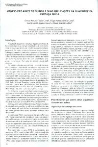
radar data may capture more vegetation stand structure information (Leckie, 1998). For example, ALOS PALSAR L-band has a longer wavelength than RADARSAT-2 C-band, and thus L-band data may capture more understory information than C-band data. As Table 2 indicates, L-band data yield better classification for FLF than C-band data because of the water component under the forest canopy. However, the radar data cannot effectively capture the different stand structures of succession stages, UPF, and LIF. Therefore, pure radar data cannot effectively provide as good classification results as TM images. Because L-band data perform relatively well in classification of FLF and AGP, combining TM and L-band data as extra bands improved FLF, SS1, and AGP classification. In contract, C-band data perform relatively well in classification of AGP; thus a combination of TM and C-band data as extra bands only slightly improve AGP classification but yield very limited improvement in classification of other land cover types. The analysis above indicates that individual radar data did not have the capability to satisfactorily classify land covers with finely detailed vegetation classes in this research. However, Table 2 indicates that PALSAR L-band data did provide relatively good separation of FLF from UPF and LIF, AGP from SS1, and SS2 from SS1 and SS3. RADARSAT-2 C-band data performed relatively well in classification of SS2 and AGP. Further analysis of the error matrices indicates that the major misclassification from radar data is in the vegetation classes, wetland, and urban. When we merged vegetation types into coarse classes, for example, merging UPF, FLF, and LIF as Forest and merging SS1, SS2, and SS3 as SS, and finally merging Forest and SS as one class, the PA and UA values were much improved, as shown in Table 4. This result implies that radar data, especially from the PALSAR L-band, are valuable for land cover classification in a coarse classification system, but not suitable for a detailed vegetation classification system. Color Composites from Different Data Fusion Methods Different data fusion methods have different capabilities in preserving spectral fidelity while improving spatial resolution. Figure 3 provides a comparison of color composites among original TM bands and different fusion results by assigning bands 4, 5, and 3 as red, green and blue, respectively, as well as radar data by assigning HH, HV, and NL as red, green and blue, respectively. Figure 3 shows that both Wavelet and HPF fusion methods preserve the spectral fidelity of the input dataset, but the HPFderived fusion result appears very noisy. The PCA- and NMM-based methods distort the spectral signatures, although these color composites seem to improve visual interpretation effects. Analysis of all color composites from the data fusion methods based on TM multispectral bands and different radar images (i.e., HH, HV, and NL images from the PALSAR L-band or the RADARSAT-2 C-band separately) yields a similar conclusion: the Wavelet fusion method best preserves spectral fidelity, followed by the HPF-based fusion method, no matter what polarization (HH, HV, or NL) image from PALSAR L-band or RADARSAT-2 C-band is used. Comparison of the color composites with their land cover classification results is valuable for better understanding the importance of preserving spectral fidelity when multisensor data are used for data fusion in quantitative analyses.
32
5
41
23
0
0
1
0
4
42
6
0
2
6
SS
AGP
WAT
WET
URB
FOR
SS
AGP
WAT
WET
URB
1
2
0
15
7
1
0
1
0
24
1
0
AGP
URB
RT
0
4
0
8
3
0
5
3
0
2
6
7
5
9
23
43
66
66
1
0
23
0
0
0
0
0
0
6
9
0
3
0
0
13
5
2
17
9
23
47
104
12
RADARSAT C-band HH, HV, and NL data
0
0
23
0
1
0
WET
PALSAR L-band HH, HV, and NL datab
WAT
c
23
15
24
26
64
60
23
15
24
26
64
60
CT
13.0
0.0
95.8
57.7
64.1
6.7
21.7
20.0
95.8
92.3
50.0
60.0
PA1
17.6
0.0
100.0
31.9
39.4
33.3
100.0
44.4
100.0
55.8
48.5
54.5
UA1
74.19
91.93
PA2
79.31
86.36
UA2
a AGP = agropasture; CT = column total; FOR = merged class of forest that includes upland, flooding, and liana forests; PA1, UA1, and OCA1 = producer’s accuracy, user’s accuracy, and overall classification accuracy based on six classes; PA2, UA2, and OCA2 = producer’s accuracy, user’s accuracy, and overall classification accuracy based on five classes in which merged FOR and SS form one class; RT = row total; SS = a merged class of secondary succession vegetation that includes initial, intermediate, and advanced succession vegetations; URB = urban; WAT = water; WET = wetland. b OCA1 = 58.49%; OCA2 = 80.19%. c OCA1 = 40.57%; OCA2 = 62.74%
6
5
0
7
0
0
9
23
36
FOR
SS
FOR
Land cover type
Table 4. A Comparison of Error Matrices Between the Classification Results from PALSAR L-Band and RADARSAT-2 C-Band Dataa
358 lu et al.
multisensor integration methods
359
Fig. 3. A comparison of color composites from TM, radar, and their fused images using different data fusion methods. A and B are TM color composites with bands 4, 5, and 3 assigned as red, green, and blue, respectively. A is the entire area, whereas B through L show an enlarged area to better illustrate the different features among the data fusion results. C is a color composite based on PALSAR L-band HH, HV, and NL. D is a color composite based on RADARSAT-2 C-band HH, HV, and NL. E–H are data fusion results from PCA, Wavelet, HPF, and NMM based on TM and PALSAR L-band HH imagery. I–L are data fusion results from PCA, Wavelet, HPF, and NMM based on TM and RADARSAT-2 C-band HH data.
69.7 86.7 83.3 47.4 75.0 57.1 80.8 87.5 73.3 100.0
66.7 86.7 83.3 57.9 75.0 57.1 73.1
OCA OKC
UPF FLF LIF SS1 SS2 SS3 AGP
PA
UPF FLF LIF SS1 SS2 SS3 AGP WAT WET URB
Land cover type
UA
69.7 68.4 66.7 60.0 75.0 70.6 72.4 100.0 91.7 85.2
71.0 68.4 71.4 57.9 69.2 75.0 73.1
75.94 0.7305
PCA
85.85 0.8413
80.66 0.7835
Data fusion based on TM and PALSAR L-band HV data 75.8 83.3 69.7 74.2 93.3 73.7 93.3 73.7 83.3 83.3 75.0 69.2 79.0 71.4 63.2 66.7 87.5 91.3 75.0 78.3 90.5 86.4 85.7 75.0 80.8 91.3 76.9 87.0
63.6 73.3 83.3 57.9 70.8 52.4 76.9
72.7 86.7 83.3 21.1 58.3 52.4 80.8 87.5 60.0 100.0
Data fusion based on TM and PALSAR L-band HH data 75.8 89.3 69.7 74.2 93.3 70.0 93.3 70.0 91.7 84.6 75.0 69.2 79.0 71.4 63.2 66.7 87.5 91.3 75.0 85.7 90.5 86.4 85.7 75.0 80.8 91.3 80.8 87.5 87.5 100.0 91.7 100.0 80.0 100.0 73.3 100.0 100.0 79.3 100.0 82.1
PA
PA
UA
HPF UA
PA
Wavelet UA
75.0 81.3 62.5 25.0 66.7 61.1 65.6 100.0 100.0 74.2
63.6 61.1 71.4 52.4 65.4 73.3 76.9
70.75 0.6721
NMM
Table 5. Comparison of Classification Results from Different Data Fusion Methods Based on TM and PALSAR L-Band HH, HV, and NL Data
360 lu et al.
87.5 80.0 100.0
69.7 86.7 75.0 52.6 70.8 52.4 76.9 91.7 80.0 100.0
WAT WET URB
OCA OKC
UPF FLF LIF SS1 SS2 SS3 AGP WAT WET URB
OCA OKC
75.47 0.725
67.7 72.2 69.2 58.8 68.0 68.8 71.4 100.0 92.3 88.5
75.94 0.7307
100.0 92.3 85.2 85.38 0.8364
100.0 1 00.0 79.3
87.5 73.3 100.0 79.72 0.7729
100.0 1 00.0 79.3
84.43 0.826
82.55 0.8045
Data fusion based on TM and PALSAR L-band NL data 72.7 85.7 75.8 75.8 93.3 70.0 93.3 66.7 83.3 76.9 75.0 81.8 79.0 68.2 73.7 70.0 83.3 90.9 79.2 90.5 90.5 86.4 81.0 77.3 80.8 91.3 80.8 91.3 87.5 100.0 91.7 100.0 80.0 100.0 73.3 100.0 100.0 79.3 100.0 82.1
87.5 80.0 100.0
66.7 80.0 83.3 52.6 66.7 52.4 76.9 87.5 73.3 100.0
87.5 60.0 100.0
73.58 0.7042
68.8 66.7 71.4 50.0 64.0 68.8 76.9 100.0 91.7 82.1
72.64 0.6934
100.0 90.0 82.1
multisensor integration methods
361
UPF FLF LIF SS1 SS2 SS3 AGP WAT WET URB
OCA OKC
UPF FLF LIF SS1 SS2 SS3 AGP
Land cover type
72.7 86.7 75.0 52.6 79.2 76.2 61.5
69.7 86.7 75.0 57.9 79.2 71.4 61.5 87.5 60.0 100.0
PA
75.00 0.7202
PCA PA
UA
PA
HPF UA
85.38 0.8365
81.60 0.7940
Data fusion based on TM and RADARSAT-2 C-band HV data 70.6 78.8 89.7 75.8 75.8 52.0 93.3 70.0 93.3 73.7 75.0 83.3 83.3 83.3 83.3 66.7 79.0 75.0 63.2 66.7 82.6 91.7 91.7 79.2 86.4 88.9 90.5 86.4 85.7 78.3 64.0 80.8 91.3 80.8 87.5
Data fusion based on TM and RADARSAT-2 C-band HH data 71.9 75.8 89.3 72.7 75.0 54.2 93.3 70.0 93.3 73.7 75.0 83.3 83.3 83.3 76.9 68.8 79.0 71.4 68.4 65.0 79.2 91.7 88.0 79.2 82.6 79.0 90.5 86.4 81.0 77.3 66.7 76.9 90.9 76.9 90.9 100.0 87.5 100.0 91.7 100.0 75.0 80.0 100.0 73.3 100.0 82.1 100.0 79.3 100.0 82.1
UA
Wavelet
51.5 93.3 83.3 36.8 45.8 57.1 65.4
57.6 93.3 83.3 36.8 58.3 47.6 69.2 87.5 86.7 95.7
PA
69.81 0.6626
NMM
68.0 63.6 62.5 31.8 64.7 66.7 54.8
67.9 66.7 58.8 36.8 66.7 76.9 56.3 100.0 92.9 84.6
UA
Table 6. Comparison of Classification Results from Different Data Fusion Methods Based on TM and RADARSAT-2 C-Band HH, HV, and NL Data
362 lu et al.
WAT WET URB
OCA OKC
UPF FLF LIF SS1 SS2 SS3 AGP WAT WET URB
OCA OKC
72.7 86.7 75.0 47.4 75.0 76.2 61.5 87.5 53.3 100.0
87.5 53.3 100.0
87.5 80.0 100.0 86.32 0.8470
100.0 100.0 79.3
91.7 73.3 100.0 82.55 0.8044
100.0 100.0 82.1
86.79 0.8522
83.02 0.8097
Data fusion based on TM and RADARSAT-2 C-band NL data 68.6 78.8 89.7 75.8 75.8 54.2 93.3 73.7 93.3 73.7 81.8 83.3 83.3 83.3 76.9 64.3 79.0 75.0 63.2 70.6 78.3 91.7 91.7 79.2 86.4 88.9 95.2 87.0 85.7 81.8 59.3 80.8 91.3 84.6 88.0 100.0 87.5 100.0 91.7 100.0 72.7 80.0 100.0 73.3 100.0 82.1 100.0 79.3 100.0 82.1
100.0 72.7 82.1
74.06 0.7091
75.00 0.7200
60.6 93.3 83.3 31.6 54.2 66.7 65.4 87.5 86.7 100.0
87.5 86.7 100.0
71.4 66.7 62.5 30.0 61.9 73.7 65.4 100.0 100.0 85.2
100.0 100.0 85.2
71.23 0.6786
68.40 0.6473
multisensor integration methods
363
364
lu et al.
Classification Results from Different Data Fusion Methods The land cover classification results from the MLC among different data fusion methods indicate that, compared to the original Landsat TM image, the Wavelet method improved land cover classification and HPF had similar OCA values; in contrast, PCA and NMM reduced classification quality. For example, the Wavelet method improved OCA by 3.3%–5.7%, HPF performed similarly, but PCA and NMM reduced OCA by 5.1%–6.1% and 7.6% –12.7%, respectively. In particular, the Wavelet fusion method improved vegetation classification accuracies, no matter which wavelengths (L-band or C-band) and which polarization options (HH or HV, or the NL image) were used. Comparing the land cover classification results (Tables 5 and 6) and the color composites (see Fig. 3) shows the importance of preserving the spectral fidelity of the TM multispectral signatures. Comparative analysis of the accuracy assessment results among different data fusion methods further indicates that Wavelet and HPF are helpful in improving vegetation classification accuracies. This finding implies that it is important to understand the role of a specific data fusion method in enhancing specific kinds of land cover types. Polarizations HH, HV, and NL perform similarly in land cover classification when they are used for data fusion with TM images, except for the NMM method. As a comparison, the error matrix (Table 7) from the Wavelet fusion result based on TM and PALSAR L-band HH shows that UPF, LIF, SS1, SS3, and AGP are especially improved, compared to the original TM image (see Table 3). A comparison of some classification results (Fig. 4) among the selected scenarios indicates that both radar images (ALOS PALSAR L-band and RADARSAT-2 C-band data in this research) cannot separate different land cover classes, except water (see Figs. 3C and 3E). Incorporation of TM and radar data provided spatial patterns of land cover distribution (see Figs. 3D and 3F) similar to the original TM image classification result (see Fig. 3B). In general, data fusion is often applied to improve spatial resolution, and thus may reduce mixed-class pixels. This spatial improvement is helpful for sites having relatively small patches of land cover, such as different stages of successional vegetation. However, due to the complex stand structure in vegetation types, especially for primary forest and advanced succession, increased spatial resolution may enlarge the spectral variation within the same land cover, as shown in Figures 3G and 3F, and thus reduce the classification accuracy. Therefore, there is a tradeoff between patch size of land covers and the spectral variation caused by improved spatial resolution. Future research should examine how different spatial resolutions affect the selection of data fusion methods and what classification algorithm is suitable for land cover classification corresponding to the fusion images. CONCLUSIONS This research indicates that a TM image provides higher land cover classification accuracy than individual radar datasets, and PALSAR L-band data provide better classification than RADARSAT-2 C-band data. Neither PALSAR nor RADARSAT data have the capability for detailed vegetation classification, but they are valuable for coarse land cover classification. When radar data are used as extra bands incorporated
25
5
2
0
0
1
0
0
0
0
UPF
FLF
LIF
SS1
SS2
SS3
AGP
WAT
WET
URB
0
0
0
0
0
0
0
0
14
1
FLF
0
0
0
0
0
0
0
11
0
1
LIF
0
0
0
2
0
2
15
0
0
0
SS1
0
0
0
0
2
21
1
0
0
0
SS2
0
0
0
0
19
0
0
0
1
1
SS3
0
0
0
21
0
0
5
0
0
0
AGP
3
0
21
0
0
0
0
0
0
0
WAT
3
12
0
0
0
0
0
0
0
0
WET
23
0
0
0
0
0
0
0
0
0
URB
29
12
21
23
22
23
21
13
20
28
RT
23
15
24
26
21
24
19
12
15
33
CT
100.0
80.0
87.5
80.8
90.5
87.5
78.9
91.7
93.3
75.8
PA
79.3
100.0
100.0
91.3
86.5
91.3
71.4
84.6
70. 0
89.3
UA
a
OCA = 85.85%; OKC = 0.8418. AGP= agropasture; CT = column total; FLF = flooding forest; LIF = liana forest; PA = producer’s accuracy; OCA = overall classification accuracy; OKC = overall kappa coefficient; RT = row total; SS1 = initial succession vegetation; SS2 = intermediate succession vegetation; SS3 = advanced succession vegetation; UA = user’s accuracy; UPF = upland forest; URB = urban; WAT = water; WET = wetland.
UPF
Land cover type
Table 7. Error Matrix Based on Wavelet Data Fusion of TM and PALSAR L-HH Dataa
multisensor integration methods
365
366
lu et al.
Fig. 4. A comparison of classification results from different scenarios. A is a classified image for the entire study area based on the original TM spectral data; the other five images show the rectangular area outlined in red in image A. B is the original TM image. C is the classified image based on PALSAR L-band HH, HV and NL data. D is based on TM and PALSAR L-band HH Wavelet fusion image. E is based on RADARSAT-2 C-band HH, HV and NL data. F is based on TM and a RADARSAT-2 C-band HH Wavelet fusion image.
into TM multispectral data, the land cover classification is not significantly improved. However, compared to the TM data, Wavelet multisensor fusion improved overall classification accuracy by 3.3%–5.7%. In contrast, performance of the HPF-based fusion method was similar to the TM image, whereas the PCA-based and NMM methods reduced overall classification accuracy by 5.1%–6.1% and 7.6% –12.7%, respectively. Different polarization options, such as HH, HV, and NL, performed similarly when they were used for multisensor data fusion. This research shows the importance of preserving spectral fidelity in improving land cover classification performance. Wavelet and HPF methods can better preserve spectral fidelity than PCA and NMM for the fusion of TM and radar data. In particular, the Wavelet multi-sensor fusion method is recommended in the moist tropical region for detailed land cover classification.
multisensor integration methods
367
ACKNOWLEDGMENTS The authors thank the National Science Foundation (grant #BCS 0850615) for funding support. Luciano Dutra thanks JAXA (AO 108) for providing the ALOS PALSAR data through its Science Program, and Mateus Batistella thanks the Canadian SOAR Program (SOAR Project #1957) for the RADARSAT-2 data used in this research. We also thank Anthony Cak for his assistance with fieldwork and Scott Hetrick for his assistance in organizing the field data. REFERENCES Ali, S. S., Dare, P. M., and S. D. Jones, 2009, “A Comparison of Pixel- and ObjectLevel Data Fusion Using Lidar and High-Resolution Imagery for Enhanced Classification,” in Innovations in Remote Sensing and Photogrammetry, Jones, S. and K. Reinke (Eds.), Berlin, Germany: Springer-Verlag, 3–17. Amolins, K., Zhang, Y. and P. Dare, 2007, “Wavelet Based Image Fusion Techniques— An Introduction, Review, and Comparison,” ISPRS Journal of Photogrammetry and Remote Sensing, 62:249–263. Blaschke, T., 2010, “Object-Based Image Analysis for Remote Sensing,” ISPRS Journal of Photogrammetry and Remote Sensing, 65:2–16. Ceamanos, X., Waske, B., Benediktsson, J. A., Chanussot, J., Fauvel, M., and J. R. Sveinsson, 2010, “A Classifier Ensemble Based on Fusion of Support Vector Machines for Classifying Hyperspectral Data,” International Journal of Image and Data Fusion, 1(4):293–307. Chander, G., Markham, B. L., and D. L. Helder, 2009, “Summary of Current Radiometric Calibration Coefficients for Landsat MSS, TM, ETM+, and EO-1 ALI Sensors,” Remote Sensing of Environment, 113:893–903. Chavez, P. S., Jr., 1996, “Image-Based Atmospheric Corrections—Revisited and Improved,” Photogrammetric Engineering and Remote Sensing, 62:1025–1036. Chen, D. and D. A. Stow, 2003, “Strategies for Integrating Information from Multiple Spatial Resolutions into Land-Use/Land-Cover Classification Routines,” Photogrammetric Engineering and Remote Sensing, 69:1279–1287. Chibani, Y., 2006, “Additive Integration of SAR Features into Multispectral SPOT Images by Means of the à trous Wavelet Decomposition,” ISPRS Journal of Photogrammetry & Remote Sensing, 60:306–314. Chitroub, S., 2010, “Classifier Combination and Score Level Fusion: Concepts and Practical Aspects,” International Journal of Image and Data Fusion, 1(2):113– 135. Congalton, R. G. and K. Green, 2008, Assessing the Accuracy of Remotely Sensed Data: Principles and Practices, 2nd ed., Boca Raton, FL: CRC Press, 183 p. Dong, J., Zhuang, D., Huang, Y., and J. Fu, 2009, “Advances in Multi-sensor Data Fusion: Algorithms and Applications,” Sensors, 9:7771–7784. Ehlers, M., Klonus, S., Astrand, P. J., and P. Rosso, 2010, “Multisensor Image Fusion for Pansharpening in Remote Sensing,” International Journal of Image and Data Fusion, 1:25–45. ERDAS, 2009, ERDAS Field Guide, Norcross, GA: ERDAS, Inc..
368
lu et al.
Estes, J. E. and T. R. Loveland, 1999, “Characteristics, Sources, and Management of Remotely-Sensed Data,” in Geographical Information Systems: Principles, Techniques, Applications, and Management, 2nd ed., Longley, P., Goodchild, M., Maguire, D. J. and D. W. Rhind (Eds.), New York, NY: Wiley, 667–675. Filippi, A. M, Brannstrom, C., Dobreva, I., Cairns, D. M. and D. Kim, 2009, “Unsupervised Fuzzy ARTMAP Classification of Hyperspectral Hyperion Data for Savanna and Agriculture Discrimination in the Brazilian Cerrado,” GIScience & Remote Sensing, 46(1):1–23. Foody, G. M., 2002, “Status of Land Cover Classification Accuracy Assessment,” Remote Sensing of Environment, 80:185–201. Franklin, S. E. and M. A. Wulder, 2002, “Remote Sensing Methods in Medium Spatial Resolution Satellite Data Land Cover Classification of Large Areas,” Progress in Physical Geography, 26:173–205. Gong, P., 1994, “Integrated Analysis of Spatial Data from Multiple Sources: An Overview,” Canadian Journal of Remote Sensing, 20:349–359. Haack, B. N. and N. D. Herold, 2007, “Comparison of Sensor Fusion Methods for Land Cover Delineations,” GIScience & Remote Sensing, 44(4):305–319. Hong, G. and Y. Zhang, 2008, “Comparison and Improvement of Wavelet-Based Image Fusion,” International Journal of Remote Sensing, 29:673–691. Jensen, J. R., 2005, Introductory Digital Image Processing: A Remote Sensing Perspective, 3rd ed., Upper Saddle River, NJ: Pearson Prentice Hall, 526 p. Jimenez, L. O., Morales-Morell, A., and A. Creus, 1999, “Classification of Hyper dimensional Data Based on Feature and Decision Fusion Approaches Using Projection Pursuit, Majority Voting, and Neural Networks,” IEEE Transactions on Geoscience and Remote Sensing, 37:1360–1366. Klonus, S. and M. Ehlers, 2007, “Image Fusion Using the Ehlers Spectral Characteristics Preservation Algorithm,” GIScience & Remote Sensing, 44(2): 93–116. Leckie, D. G., 1998, “Forestry Applications Using Imaging Radar,” in Principles and Applications of Imaging Radar (Manual of Remote Sensing, 3rd ed., Vol. 2), Henderson, F. M. and A. J. Lewis (Eds.), New York, NY: Wiley, 437–509. Lee, J. S., Jurkevich, I., Dewaele, P., Wambacq, P., and A. Oosterlinck, 1994, “Speckle Filtering of Synthetic Aperture Radar Images: A Review,” Remote Sensing Reviews, 8:313–340. Lefsky, M. A. and W. B. Cohen, 2003, “Selection of Remotely Sensed Data,” in Remote Sensing of Forest Environments: Concepts and Case Studies, Wulder, M. A. and S. E. Franklin (Eds.), Boston, MA: Kluwer, 13–46. Lemeshewsky, G. P., 1999, “Multispectral Multisensor Image Fusion Using Wavelet Transforms,” in Visual Image Processing: VIII Proceedings of SPIE, Vol. 3716, Park, S. K. and R. Juday (Eds.), Bellingham, WA: International Society for Optics and Photonics, 214–222. Li, S., Li, Z., and J. Gong, 2010, “Multivariate Statistical Analysis of Measures for Assessing the Quality of Image Fusion,” International Journal of Image and Data Fusion, 1:47–66. Lillesand, T. M. and R. W. Kiefer, 2000, Remote Sensing and Image Interpretation, 4th ed., New York, NY: Wiley, 724 p.
multisensor integration methods
369
Lu, D., Batistella, M., and E. Moran, 2007, “Land-Cover Classification in the Brazilian Amazon with the Integration of Landsat ETM+ and RADARSAT Data,” Inter national Journal of Remote Sensing, 28(24):5447–5459. Lu, D., Batistella, M., Moran, E., and E. E. de Miranda, 2008, “A Comparative Study of Landsat TM and SPOT HRG Images for Vegetation Classification in the Brazilian Amazon,” Photogrammetric Engineering and Remote Sensing, 70:311–321. Lu, D., Mausel, P., Brondízio, E. S., and E. Moran, 2002, “Assessment of Atmospheric Correction Methods for Landsat TM Data Applicable to Amazon Basin LBA Research,” International Journal of Remote Sensing, 23:2651–2671. Lu, D. and Q. Weng, 2007, “A Survey of Image Classification Methods and Techniques for Improving Classification Performance,” International Journal of Remote Sensing, 28:823–870. Lucas, R. M., Cronin, N., Moghaddam, M., Lee, A., Armston, J., Bunting, P., and C. Witte, 2006, “Integration of Radar and Landsat-Derived Foliage Projected Cover for Woody Growth Mapping, Queensland, Australia,” Remote Sensing of Environment, 100:388–406. Mausel, P., Wu, Y., Li, Y., Moran, E., and E. Brondízio, 1993, “Spectral Identification of Succession Stages Following Deforestation in the Amazon,” Geocarto International, 8:61–72. McNairn, H., Champagne, C., Shang, J., Holmstrom, D., and G. Reichert, 2009, “Integration of Optical and Synthetic Aperture Radar (SAR) Imagery for Delivering Operational Annual Crop Inventories,” ISPRS Journal of Photogrammetry and Remote Sensing, 64:434–449. Moran, E. F., 1981, Developing the Amazon, Bloomington, IN: Indiana University Press, 292 p. Moran, E. F., and E. S. Brondízio, 1998, “Land-Use Change after Deforestation in Amazônia,” in People and Pixels: Linking Remote Sensing and Social Science, Liverman, D., Moran, E. F., Rindfuss, R. R., and P. C. Stern (Eds.), Washington, DC: National Academies Press, 94–120. Moran, E. F., Brondízio, E. S., Mausel, P., and Y. Wu, 1994, “Integrating Amazonian Vegetation, Land Use, and Satellite Data,” Bioscience, 44:329–338. ndi Nyoungui, A., Tonye, E., and A. Akono, 2002, “Evaluation of Speckle Filtering and Texture Analysis Methods for Land Cover Classification from SAR Images,” International Journal of Remote Sensing, 23:1895–1925. Pohl, C. and J. L. van Genderen, 1998, “Multisensor Image Fusion in Remote Sensing: Concepts, Methods, and Applications,” International Journal of Remote Sensing, 19:823–854. Rogan, J., Franklin, J., Stow, D., Miller, J., Woodcock, C., and D. Roberts, 2008, “Mapping Land-Cover Modifications over Large Areas: A Comparison of Machine Learning Algorithms,” Remote Sensing of Environment, 112: 2272–2283. Rosenqvist, A., Shimada, M., Ito, N., and M. Watanabe, 2007, “ALOS PALSAR: A Pathfinder Mission for Global-Scale Monitoring of the Environment,” IEEE Transactions on Geoscience and Remote Sensing, 45:3307–3316. Solberg, A. H. S., Taxt, T., and A. K. Jain, 1996, “A Markov Random Field Model for Classification of Multisource Satellite Imagery,” IEEE Transactions on Geoscience and Remote Sensing, 34:100–112.
370
lu et al.
Vrabel, J., 1996, “Multispectral Imagery Band Sharpening Study,” Photogrammetric Engineering & Remote Sensing, 62(9):1075–1083. Welch, R. and M. Ehlers, 1987, “Merging Multiresolution SPOT HRV and Landsat TM Data,” Photogrammetric Engineering & Remote Sensing, 53(3):301–303. Wulder, M. A., Franklin, S. E., White, J. C., Linke, J., and S. Magnussen, 2006, “An Accuracy Assessment Framework for Large-Area Land Cover Classification Products Derived from Medium-Resolution Satellite Data,” International Journal of Remote Sensing, 27:663–683. Zhang, J., 2010, “Multisource Remote Sensing Data Fusion: Status and Trends,” International Journal of Image and Data Fusion, 1:5–24.