A Comparison of Parametric and Nonparametric Approaches to ROC Analysis of Quantitative Diagnostic Tests KARIM 0. HAJIAN-TILAKI, PhD, JAMES A. HANLEY, PhD, LAWRENCE JOSEPH, PhD, JEAN-PAUL COLLET, PhD Receiver operating characteristic (ROC) analysis, which yields indices of accuracy such as the area under the curve (AUC), is increasingly being used to evaluate the performances of diagnostic tests that produce results on continuous scales. Both parametric and nonparametric ROC approaches are available to assess the discriminant capacity of such tests, but there are no clear guidelines as to the merits of each, particularly with non-binormal data. Investigators may worry that when data are nonGaussian, estimates of diagnostic accuracy based on a binormal model may be distorted. The authors conducted a Monte Carlo simulation study to compare the bias and sampling variability in the estimates of the AUCs derived from parametric and nonparametric procedures. Each approach was assessed in data sets generated from various configurations of pairs of overlapping distributions; these included the binormal model and non-binormal pairs of distributions where one or both pair members were mixtures of Gaussian (MG) distributions with different degrees of departures from binormality. The biases in the estimates of the AUCs were found to be very small for both parametric and nonparametrlc procedures. The two approaches yielded very close estimates of the AUCs and of the corresponding sampling variability even when data were generated from non-binormal models. Thus, for a wide range of distributions, concern about bias or imprecision of the estimates of the AUC should not be a major factor in choosing between the nonparametric and parametric approaches. Key words: ROC analysis; quantitative diagnostic test; comparison, parametric; binormal model; LABROC; nonparametric procedure; area under the curve (AUC). M e d Decis Making 1997;17:94-102)
During the past ten years, receiver operator characteristic (ROC) analysis has become a popular method for evaluating the accuracy/performance of medical diagnostic tests.1-3 The most attractive property of ROC analysis is that the accuracy indices derived from this technique are not distorted by fluctuations caused by the use of an arbitrarily chosen decision “criterion” or “cutoff.“4-8 One index available from an ROC analysis, the area under the curve”’ (AUC), measures the ability of a diagnostic
test to discriminate between two patient states, often labelled “diseased” and “non-diseased.” The AUC has been of considerable interest as a summary measure of accuracy because of its meaningful interpretation.“’ Initially, ROC methods were confined to tests interpreted on rating scales and analysis was typically carried out using the binormal model. 9,10 However, they are now becoming increasingly popular for evaluating the performances of quantitative diagnostic tests with numerical results recorded directly on continuous s c a l e s . 1 , 2 , 3 , 1 1 Both parametric and nonparametric procedures can be used to derive an AUC index of accuracy for such diagnostic tests. However, Goddard and Hinberg12 warned that if the distribution of raw data from a quantitative test is far from Gaussian, the AUC [and corresponding standard error (SE)] derived from a directly fitted binormal model can be seriously distorted. This occurs because one fits a mean and standard deviation to the raw data for the diseased and non-diseased patients separately. One way to avoid the possible distortion is to use Metz’s adaptation of the binormal model, previously used with rating data, 9,13-15 with
Received February 17, 1995, from the Department of Epidemiology and Biostatistics, McGill University (KOH-T, JAH, LJ, JPC); the Division of Clinical Epidemiology, Royal Victoria Hospital (JAH); the Division of Clinical Epidemiology, Montreal General Hospital (LJ); and the Division of Clinical Epidemiology, Jewish General Hospital (PC); all in Montreal, Quebec, Canada. Revision accepted for publication July 17, 1995. Supported by an operating grant from the Natural Sciences and Engineering Research Council of Canada and the Fonds de la recherche en Sante du Quebec. Address correspondence and reprint requests to Dr. Hanley: Department of Epidemiology and Biostatistics, McGill University, 1020 Pine Avenue West, Montreal, PQ Canada H3A lA2. e-mail: (
[email protected]). 94
VOL 17/NO 1, JAN-MAR 1997 laboratory-type data.’ Metz et al. implemented the binormal model in the LABROC software. 16 The procedure first discretizes the continuous data and then uses the categories as ratings in the ROCFIT procedurel6 to obtain the maximum-likelihood estimates (MLE) of the two relevant parameters of the binormal model. From them it calculates the AUC and the corresponding SE. When the data are continuous and appear to be non-Gaussian, many users will find the nonparametric approach17-19 ” to estimating the AUC more appealing than using the binormal model, since they may worry that estimates of diagnostic accuracy based on a binormal model will be distorted. However, nonparametric area estimates will tend to underestimate the AUCs for rating data,7,20 in particular when ROC operating points are not well spread out along the ROC curve. Moreover, this method does not yield a smooth estimate of the entire ROC curve. 21 1 The variance of the nonparametric estimates of the AUC can be estimated entirely nonparametrically 18,19 or using an exponential approximation.’ Recently, Obuchowski22 found that the exponential approximation underestimates the empirical standard error of the nonparametric AUC for rating data when the “ratings” begin as continuous data with a binormal distribution and when the ratio of the standard deviations (SDS) of the two distributions is greater than 2. However, in practice the data might arise from a non-binormal model. In summary, the statistical behaviors of the AUC estimates derived from the parametric and nonparametric approaches have not been investigated for quantitative diagnostic test results, and there are no general guidelines for choosing one approach over the other. Thus, we conducted a broad numerical investigation to compare the statistical behaviors of the estimates of the AUC derived from parametric and nonparametric procedures.
Methods DATA GENERATION As is shown in the leftmost columns of tables 1 and 2, we generated continuously distributed data with sample sizes of R = 40 for diseased and R = 40 for non-diseased from various pairs of overlapping distributions with various degrees of separation; sample sizes of n = lOO/lOO were also investigated. Overall, 1,000 data sets were generated for each configuration studied. Binormal data. First, we generated continuously distributed data from two overlapping Gaussian distributions, i.e., {G, G) pairs for the “non-diseased” and “diseased’ patients with different degrees of
Parametric and Nonparametrlc ROC Analysis
l
95
separation ( A U C = 0.60, AUC = 0.75, AUC = 0.90) and with various ratios of SDs of distributions for the non-diseased to diseased (l:l, 1:1.4, 1:2 and 1:3), yielding in all 12 configurations of pairs. Non-binormal data. Data were also generated from various configurations of non-binormal pairs, where one or both members of the pairs were mixtures of Gaussian (MG) distributions: (G, MGskewed or bimodal) pairs or {MG-skewed, MGskewed) pairs. In all, as is shown in figures 1 and 2, 18 configurations of non-binormal pairs with various degrees of skewness and separation were used to generate data. We calculated how often the hypothesis of normality would be rejected with such distributions. For sample sizes of 40, the hypothesis was rejected by the Wilks’ test employed by SAS in 34% of the data sets from the moderate-skew distributions and 67% of those from high-skew distributions. For sample sizes of 100, the corresponding percentages were 59 and 97. To some, the range of distributions shown in figures 1 and 2 may seem limited. However, one can apply many monotonic transformations to the separator axis, thereby effectively covering a broader range of possibilities of non-binormal data. An example of how both distributions are converted to non-normal pairs is shown in the last row of figure 1. Each pair was generated by mapping the (-03, +w) scale used in row 2 into the (0, 11 scale by applying the transformation exp(X)/ll + exp(X11. Notice, however, that although such monotonic transformations may radically change the shapes of the distributions, they do not change the ROC curve when applied to both distributions. 2,5,13 Few of the articles in the quantitative diagnostic test literature show the distributions of raw data. In those that do, the distributions of biomarkers for diseased patients are often positively skewed. For example, Goddard and Hinberg12 reported the histograms of different biomarkers for five types of cancer; the distributions for cancer patients were skewed or bimodal. Linnet11 also showed examples where the distributions of serum bilirubin and fasting serum bile acids for diseased patients were positively skewed while the reference distribution was approximately normal. Empirically, there is considerable evidence that the binormal model used for rating data needs to include more variation for diseased patients,’ i.e., the ratio of SDs of distribution for diseased to non-diseased patients is higher than 1. Based on this empirical evidence, we included the range of ratios of SDs from 1:l to 1:3. We chose mixtures of Gaussian distributions for diseased patients since the distribution may contain unidentified disease subtypes. Thus, we allow for more variation for the diseased than the non-diseased patients.
96
l
Hajian-Tllaki, Hanley, Joseph, Collet
MEDICAL DECISION MAKING
FIGURE 1. Non-binormal
distributions used to generate data sets, with the distribution for non-diseased (broken lines) chosen to be Gaussian. The distributions for diseased (solid lines) were formed from mixtures of two Gaussian distributions to create moderate right skew (top row), very right skew (second row), a bimodal distribution third row), and moderate left skew (fourth row). Each pair of the last row was generated by mapping the t-q +4 scale used in row 2 into the (0, 1) scale by applying the transformation exptX)/[l + expcY)I. The distributions in this last row were not used in the simulations because they would give the same results as the distributions in the second row. The degrees of separation were low AUC = 0.60 (leftmost column), moderate AUC = 0.75 (middle column), and high AUC = 0.90 (rightmost column).
STATISTICAL ANALYSIS
Each generated data set underwent two analyses: 1) nonparametric ROC analysis using the raw data, and 2) parametric ROC analysis of the categorized data via the LARROC approach. Nonparametric approach. The nonparametric estimate of the AUC was calculated directly from the raw data using the Wilcoxon-Mann-Whitney twosample statistic; the SE of the AUC was calculated by DeLong et al.‘s method.” Parametric ROC analysis: Each data set was analyzed via Metz's LABROC procedure. 16 The program categorizes the data according to a data-dependent rule that tries to ensure the greatest possible uniformity of spread of ROC operating points. We stipulated a maximum of ten data categories for sample sizes of 40/40 and 20 data categories for lOO/lOO (these are the default numbers of data’ categories used in the LARROC software). The program then fits a two-parameter binormal ROC curve by the method of maximum-likelihood estimation (MLE) using the categories as ratings. From the two parameters of this binormal model, it calculates an estimate of the ALJC and its SE, which we call the “calculated” SE.
\!’
A A ” i
FIGURE 2. Additional non-binormal distributions used to generate data sets with non-Gaussian distributions for both nondiseased and diseased. Distributions for both non-diseased (broken lines) and diseased (solid lines) were formed from mixtures of two Gaussian distributions to create moderate left skew (first row) and moderate right skew (second row). The degrees of separation were: low AUC = 0.60 (leftmost column), moderate AUC = 0.75 (middle column), and high AUC = 0.90 (right most column).
VOL 17/NO 1, JAN-MAR 1997
Parametric and Nanparametric ROC Analysis
l
97
Table l a 0 Comparison of Parametric and Nonparametric Approaches with Respect to Bias of the Estimates of AUC and the Corresponding Standard Errors in 1,000 Data Sets Generated from Various Configurations of the Binormal Model, N = 4O/40
Degree of Accuracy (True Index)
Ratio of SDS D:NDf
100 x Bias of Est AUC
Parametric* 100 x SE (Est AUC) Emoir
(4
61
Nonparametric
Ave Est
100 x Bias of Est AUC
63
6’)
(E’)
100 x SE (Est AUC) Emoir
Ratio of SEs
Ave Est Delano
F) -
(W(B) (W(E)
(E)/(B) W(C)
Low AUC = 0.60
1 1.4 2 3
0.5 -0.2 -0.3 -0.3
6.69
6.95 6.86 8.71
6.22 6.30 6.51 8.77
-0.1 -0.1 -0.1 -0.2
6.42 6.47 6.59 6.82
6.38 6.42 8.59 6.85
0.93 0.91 0.96 1.01
0.99 0.99 1 .oo 1 .oo
0.98 0.93 0.96 1.02
1.02 1.02 1.01 1.01
Moderate AUC = 0.75
1 1.4 2 3
0.9 0.8 0.3 -0.1
5.68 5.89 6.11 8.15
5.26 5.33 5.58 5.89
0.1 -0.0 0.0 0.1
5.53 5.60 5.78 6.03
5.42 5.49 5.67 5.93
0.93 0.90 0.91 0.96
0.98 0.98 0.98 0.98
0.97 0.95 0.95 0.98
1.03 1.03 1.02 1.01
High AUC = 0.90
1 1.4 2 3
0.7 0.6 0.6 0.4
3.35 3.46 3.75 4.19
3.24 3.31 3.46 3.76
0.0 -0.1 0.0 0.1
3.51 3.62 3.83 4.10
3.34 3.42 3.59 3.83
0.97 0.96 0.93 0.90
0.95 0.94 0.94 0.93
1.05 1.05 1.02 0.96
1.03 1.03 1.03 1.02
*Ten data categories were used in fitting the binormal model. tD = diseased; ND = non-diseased; Est = estimate; Ave = average; Empir = empirical; SE = standard error; SD = standard deviation.
Table 1 b s Comparison of Parametric and Nonparametric Approaches with Respect to Bias of the Estimates of AUC and the Corresponding Standard Errors in 1,000 Data Sets Generated from Various Configurations of the Binormal Model, N = lOO/lOO Ratio of SEs
Nonparametric
Parametric* 100 x Degree of Accuracy (True Index) Low AUC = 0.60
Moderate AUC = 0.75
100 x Bias of Ratio of SDS Est AUC D:NDt (A)
100 x SE (Est AUC) Empir (B)
Ave Est (C)
Bias of Est AUC (D)
100 x SE (Est AUC) Empir (E)
Ave Est Delong (0 4.00 4.04 4.15 4.32
1 .oo 1 .oo 1.03 1.04
1.03 1.03 1.02 1.02
0.99 0.99 1.02 1.04
1.02 1.02 1.02 1.03
1.03 1.03 1.02 1 .Ol
1.01 0.99 1 .oo 1.03
1.02 1.02 1.02 1.02 1.01 1.01 1.01 1.02
(C)/(B) (WE) (W(B) (V(C)
1 1.4 2 3
0.2 0.0 -0.1 -0.2
3.91 3.97 3.97 4.08
3.91 3.96 4.07 4.21
-0.1 -0.1 -0.1
-0.1
3.89 3.94 4.05 4.22
1 1.4 2 3
0.5 0.3 0.0 -0.2
3.29 3.39 3.50 3.60
3.34 3.39 3.52 3.68
0.0 -0.1 0.0 0.0
3.31 3.37 3.50 3.71
3.41 3.48 3.58 3.75
1.02 1.00 1 .Ol 1.02
High
1
0.2
1.99
2.10
-0.1
2.07
2.13
1.06
1.03
1.04
AUC = 0.90
1.4
0.1
2.03
2.16
-0.1
2.15
2.19
1.06
1.02
1.08
2 ” 3
0.0 -0.1
2.23 2.50
2.28 2.44
-0.1 -0.0
2.28 2.47
2.31 2.48
1.02 0.98
1 .Ol 1 .oo
1.02 0.99
*20 data categories were used in fitting the binormal model. tD = diseased; ND = non-diseased; Est = estimate; Ave = average: Empir = empirical; SE = standard error; SD = standard deviation. COMPARISON OF STATISTICAL BEHAVIORS OF PARAMETRIC AND NONPARAMETRIC ESTIMATES
The biases in the estimates of the ALJC (i.e., the difference between the average of the 1,000 estimates of the AUC and the true value) from the parametric and nonparametric approaches were calculated and compared. The magnitude of the bias in the estimates of the AUC and the absolute discrepancy between individual estimates of the AUC
from the two approaches were used to judge the impact of model mis-specification. The SD of the 1,000 estimates of the AUC derived from one approach was compared with the corresponding SD of the 1,000 AUC estimates from the other approach. For each approach, this SD (which we call the empirical SE) was also compared with the average of the 1,000 calculated SEs. In addition, we compared the average calculated SE of the AUC derived from the binormal model with that calcu-
98 0 Hajian-Tilaki, Hanley, Joseph, Collet
MEDICAL DEClSlON MAKING
Table 2a 0 Comparison of Parametric and Nonparametric Approaches with Respect to Bias of the Estimates of AUC and the Correspondlng Standard Errors in 1,000 Data Sets Generated from Various Configurations of Non-binormal Models, N = 40/40 Parametric* 100 x SE (Est AUC) Empir (B)
Ave Est (C)
8.22
8.37
0.2
5.87
8.48
1.02
1.10
0.94
1.02
5.24
5.29
0.3
5.15
5.45
1.01
1.08
0.98
1.03
3.11
3.18
0.2
3.29
3.21
1.02
0.98
1.06
1 .oe
0.2
4.93
8.83
0.3
4.77
6.78
1.34
1.42
0.97
1.02
2.1
4.50
5.38
0.3
4.48
5.59
1.20
1.25
1 .oo
1.04
.O.Q
3.04
3.35
0.2
3.27
3.41
1.10
1.04
1.08
1.02
1.1
4.58
8.88
0.2
3.95
8.82
1.48
‘1.73
0.87
1.02
2.2
3.38
5.48
0.1
3.73
5.74
1.82
1.54
1.10
1.05
0.9
2.57
3.34
0.1
2.93‘
3.41
1.30
1.18
1.14
1.02
-1.3
6.32
8.48
0.0
5.91
8.57
1.03
1.11
0.94
1 .Ol
-0.5
5.59
5.81
-0.2
5.21
5.88
1.04
1.13
0.93
1 .Ol
0.8
3.71
3.72
0.2
3.69
3.84
1 .oo
1.04
0.99
1.03
0.4
8.07
6.24
0.0
5.53
6.38
1.03
1.15
0.91
1.02
1.3
5.22
5.32
0.1
4.84
5.53
1.02’
1.14
0.93
1.04
1.1
3.23
3.61
0.0
3.54
3.79
1.12
1.07
1.10
1.05
0.5
8.10
6.21
0.2
5.61
6.35
1.02
1.13
0.92
1.02
1.1
5.16
5.22
0.2
4.88
5.39
1.01
1.11
0.94
1.03
0.9
3.14
3.34
0.1
3.28
3.44
1.08
1.05
1.04
1.03
100 x Distributions Degree of Bias of for ND Accuracy Est AUC (True Index) 8, Dt (A) ND: G Low D:MG& AUC = 0.805 1.2 moderate Moderate AUC = 0.753 1.5 skew High (nght) AUC = 0.907 0.8 ND: G 0: MG 81 very skew (right) ND: G 0: MO & bimodal
ND: G 0: MG & left skew
ND: MG 0: MG both left skew
ND: MG 0: MG both right skew
Low AUC = 0.808 Moderate AUC = 0.752 High AUC = 0.898 Low AUC = 0.605 Moderate AUC = 0.751 High AUC = 0.900 Low AUC = 0.807 Moderate AUC = 0.741 High AUC ; 0.891 Low AUC = 0.809 Moderate AUC = 0.750 High AUC = 0.885 Low AUC = 0.807 Moderate AUC = 0.755 High AUC = 0.898
100 x Bias of Est AUC (D)
Nonparametric 100 x SE (Est AUC) Ave Est Empir Delong (E) (P)
Ratio of S,Es
(W(B) (P)/(E) (E)/(B) (WC)
*The binormal model was fitted using ten data categories. tND = non-diseased; D = diseased; G = Gaussian; MG = mixture of Gaussian; SE = standard error; Empir = empiriial.
lated for the nonparametric estimate using DeLong’s method.
erate 23,24 4 data sets. In other words, the MLE iteration procedure converged for all data sets. PERFORMANCE WITH BINORMAL DATA
Results Table 1 compares the results from the parametric and nonparametric approaches when data are generated from the binormd model, while table 2 compares the results for non-binormal data. When fitting the binormal model, there were no degen-
Columns (A) and (D) in tables la and lb show that when data were generated from a pair of Gaussian distributions both the parametric and the nonparametric approaches yielded close to unbiased estimates of the AUC. The biases were 50.9% and S0.2%, respectively, for the sample sizes of 40/40;
VOL 17/NO 1, JAN-MAR 1997
Parametric and Nonparametric ROC Analysis
l
99
Table 2b 0 Comparison of Parametric and Nonparametric Approaches with Respect to Bias of the Estimates of AUC and the Corresponding Standard Errors in 1,000 Data Sets Generated from Various Configurations of Non-binormal Models, N = 100/100 Parametric* 100 x SE (Est AUC) Empir (B)
Ave Est (C)
3.55
3.98
0.0
3.81
4.08
1.12
1.13
1.02
1.03
3.11
3.37
0.1
3.17
3.44
1.08
1.08
1.02
1.02
1.91
2.07
0.1
1.96
2.08
1.08’
1.05
1.03
1 .oo
2.3
2.92
4.10
0.1
2.97
4.25
1.40
1.43
1.02
1.04
1.6
2.61
3.41
0.1
2.77
3.25
1.31
1.27
1.06
1.03
0.3
1.83
2.18
0.1
1.95
2.17
1.19
1.11
1.07
1 .oo
1.2
2.67
4.13
0.0
2.42
4.28
1.55
1.77
0.91
1.04
2.0
2.19
3.44
0.0
2.27
3.61
1.57
1.59
1.04
1.05
0.5
1.53
2.18
0.1
1.73
2.15
1.41
1.24
1.13
1 .oo
-1.2
3.69
4.05
0.0
3.86
4.13
1.10
1.13
0.99
1.02
-0.7
3.26
3.63
-0.1
3.21
3.69
1.11
1.15
0.98
1.02
0.4
2.16
2.39
0.3
2.16
2.44
1.11
1.13
1 .oo
1.02
0.4
3.55
3.90
0.0
3.38
4.01
1.10
1.19
0.95
1.03
0.9
2.99
3.36
0.1
2.97
3.48
1.12
1.17
0.99
1.04
0.8
1.93
2.31
0.0
2.09
2.39
1.20
1.14
1.08
1.03
0.3
3.60
3.89
0.1
3.46
3.98
1.06
1.15
0.96
1.02
0.6
3.01
3.30
0.1
2.96
3.39
1.10
1.15
0.98
1.03
0.4
1.93
2.14
0.1
1.98
2.18
1.11
1.10
1.03
1.02
100 x Distributions Degree of Bias of for ND Accuracy Est AUC (True index) 8 Dt (A) Low ND: G D:MG& AUC = 0.605 1.2 moderate Moderate skew AUC = 0.753 0.9 High (nght) 0.2 AUC = 0.907 ND: G D: MG & very skew (right) ND: G D: MO &
ND: G D:MG& left skew
ND: MO D: MO both left skew
ND: MG D: MG both right skew
Low AUC = 0.606 Moderate AUC = 0.752 High AUC = 0.896 Low AUC = 0.605 Moderate AUC = 0.751 High AUC = 0.900 Low AUC = 0.607 Moderate AUC = 0.741 High AUC = 0.891 Low AUC = 0.609 Moderate AUC = 0.750 High AUC = 0.665 Low AUC = 0.607 Moderate AUC = 0.755 High AUC = 0.898
Nonparametric 100 x 100 x SE Bias of (Est AUC) Ave Est Est AUC Emoir Delona (i (D) tP) -
Ratio of SEs
(C)/(B) (W(B) (E)/(B) (W(C)
*The binormal mqClel was fitted using 20 data categories. PND = non-diseased: D = diseased: G = Gaussian: MG = mixture of Gaussian; SE = standard error; Empir = empirical.
(0.5% and =O.l%, respectively, for those of 1 0 0 / 1 0 0
Estimated SE versus empirical SE of estimates of the AUC. For the parametric approach, the average calculated SE from the binormal model [Column (C) in table lb] is close to the actual (empirical) variation [Column (B)]. The ratio of SEs for Column 02) to Column (B) ranged from 0.91 to 1.01 over the configurations studied for the 40/40 case and from 0.98 to 1.06 for the 100/100 case. DeLong et al.‘s nonparametric estimate of the SE [Column ( F ] is close to the actual (empirical) varia-
tion of the Wilcoxon-Mann-Whitney statistic [column (E)] for all configurations studied: the ratio of SEs for Column (F) to Column (E) ranged from 0.93 to 1 for the 40/40 case and from 1 to 1.03 for the 100/100 case.
Sampling variability of parametric and nonparametric estimates. With sample sizes of 1 0 0 / 1 0 0 the empirical variation of the nonparametric AUC, Column (E), tended to be slightly greater than the model-based estimates, Column (B). The corresponding ratios ranged from 0.99 to 1.06; these
100
l
Hajian-Tilaki, Hanley, Joseph, Collet
ratios ranged from 0.93 to 1.05 with 40/40. Also, the estimated SEs of the
sample sizes of nonparametric estimates, obtained by DeLong et al’s method, were slightly greater than those of the parametric model for the 40/40 and the 100/100 cases (the ratio of SEs ranging from 1.01 to 1.03). PERFOBMANCEWITHNON-BINOBMALDATA Bias in the estimates of the AUC. Columns (A) and (D) in tables 2a and 2b show that the biases in the parametric and nonparametric estimates of the AUC are both very small. Nonparametric estimates of the AUC were virtually unbiased [the largest bias across column (D) with both sample sizes was 0.3% (or 0.003 in absolute value)]. The bias in the estimates of the AUC from fitting the binormal model to nonbinormal data was usually less than 1%. With the parametric approach, the greatest bias, 2.3% , occurred when the distribution for the diseased was highly skewed and the sample sizes were 100/100 (true AUC = 0.6061. The results were similar when the distribution for the non-diseased patients was Gaussian and the distribution for the diseased patients was bimodal and there was a moderate degree of separation between them (true AUC = 0.75). We also examined the discrepancy between the parametric and nonparametric estimates of the AUC in each of the 1,000 individual data sets. In the case of the most serious departure from normality (bimodal form), the absolute discrepancy between the two estimates of the AUC was always less than 0.05; in 99% of data sets the discrepancy was less 0.04, and in 52% the discrepancy was less than 0.02. Sampling variability. The binormal estimates of the calculated SE of the AUC and DeLong et al’s estimate of the SE of the nonparametric AUC almost always overestimated the true SEs: by -2% to 73% in the 40/40 case and by 5% to 77% in the lOO/lOO case. The greatest overestimation occurred when the distribution for the diseased patients was Gaussian and that for the non-diseased patients was bimodal. While it is difficult to know what to expect with the parametric SE when the data do not fit the model, we were surprised to find that overestimation is just as large with the nonparametric SE. With both the 40/40 and the lOO/lOO cases, the empirical variation of the AUCs from parametric fits was usually smaller than that from the nonparametric approach when the AUC was 0.90; but the pattern was less clear when the AUC was 0.75 or 0.60. However, the average nonparametric estimated SE of the AUC (DeLong et al’s method) was equal to or slightly greater than the corresponding value using the binormal model (the ratios ranged from 1 to 1.051. Overall, the parametric and nonparametric
MEDICAL DECISION MAKING
approaches yielded very similar estimates of the AUC and of the corresponding sampling variability.
Discussion This numerical investigation was conducted with a wide range of parameters of diagnostic accuracy and various degrees of departures from binormality. The results also apply to all pairs of distributions that could be converted, by some monotonic transformation, to those we studied. The findings should help users to understand the consequences of using either a parametric or a nonparametric approach to ROC analysis of the accuracies of diagnostic tests that yield results on continuous scales. Investigators may worry that when data are nonGaussian, estimates of diagnostic accuracy based on a binormal model could be distorted. However, our results show that any biases in the estimates of the AUC derived from both parametric and nonparametric approaches are very small. The results suggest that the AUC is robust to departures from binormality if one uses the binormal model as implemented in the LARROC program. However, other indices, such as true-positive fraction at a specific false-positive fraction point, might be more sensitive to departures from binormality.25 Since the bias in the nonparametric and modelbased estimates of the AUC is for all practical purposes negligible, the choice should depend on which approach yields greater precision of the estimate of diagnostic accuracy (AUC) and on the feasibility of each approach. Generally, if one uses a correct model, one might expect more precision using a model-based estimate of diagnostic accuracy than using a nonparametric estimate. This hypothesis is supported by the results of the parametric estimates of the AUC derived from data generated from various configurations of {G, G) pairs with sample sizes of 100/100 The model-based estimates of the AUC tended to have slightly less empirical variation than the nonparametric estimates. However, with sample sizes of 40/40 our investigation showed that with binormal data, there was no such gain, presumably because of the presence of the considerable noise with these small sample sizes. With non-binormal data, the gain in precision is achieved only when the AUC = 0.90, since in this situation there is less room for error in ROC space from fitting an incorrect model. Although we compared the two approaches on the basis of both their empirical SEs and their calculated SEs, we are more interested in the empirical SEs, since the calculated SEs might be distorted by fitting an incorrect model. For non-binormal data, our results show that the calculated SEs of both approaches tended to be greater than the
VOL 17/NO 1, JAN-MAR 1997
corresponding empirical SEs. We have shown elsewhere” that, for a given sample size, if one wishes to use the parametric model used in LABROC, some gain in the precision of measures of diagnostic accuracy can be achieved by increasing the number of data categories. The greatest gain in precision (10%) could be obtained when the number of data categories was increased from five to ten. When the number of data categories was further increased, the additional gain in precision was sma11. 25 In terms of practicality, the parametric approach has several advantages: The LABROC program is available in the public domain for several computer platforms. The LABROC procedure (which uses ten or 20 data categories with sample sizes of 40/40 or more) almost always converges, because the categorization algorithm used in this program automatically ensures the largest possible uniformity of the spread of ROC operating points for continuous data. This is in contrast to the poorer performance of ROCFIT16 with rating data, where, in one investigation, 22 some 16% to 37% of data sets containing rating data with small numbers of rating categories were degenerate. Moreover, one can obtain a smooth ROC curve by fitting a parametric model. On the other hand, the nonparametric approach avoids making distributional assumptions, which can be perceived as somewhat restrictive. This approach also has the appeal that the AUC is easy to calculate and is obtainable even for small sample sizes. The disadvantage is that the method does not yield a smooth estimate of the entire ROC curve. While one might consider the ease of use of the exponential approximation of the SE of the nonparametric AUC to be an advantage, based on our results, we recommend DeLong et al.‘s estimate of the SE for the nonparametric AUC, which is based directly on the Wilcoxon-Mann-Whitney statistic. However, the software is not currently widely available. Overall, the results of our simulation study suggest that for a broad range of pairs of distributions containing mixtures, parametric and nonparametric approaches yield very close estimates of diagnostic accuracy (AUC) and the corresponding precision. Thus, concern about bias or precision of the estimates of the AUC should not be a major factor in choosing between the nonparametric and parametric approaches. What are the possible reasons for the similarity of the results from the two approaches? One reason could be that we did not study a sufficiently wide range of possibilities. However, we believe that the explanation has more to do with the fact that both procedures begin by replacing the original data by their ranks. In the purely nonparametric approach,
Parametric and Nonparametric ROC Analysis
l
101
the rank transformation obliterates the original distributions. In the LABROC approach, and to a lesser extent in procedures such as ROCFIT16 and RSCORE,10 the categorization procedure used is a coarser version of ranking, and a binormal model is fitted to these categories. Thus, this procedure is essentially “semi-parametric.” There have been similar findings concerning the effect of rank transformation in two allied situations26-28 Conover and Iman26 showed that the ranking procedure reduces the probability of misclassification in discriminant analysis with non-binormal data. O’Gorman and Woolson27 reported that the use of rank transformation increases the chance of correctly identifying important non-Gaussian explanatory variables in discriminant analysis. In another paper,” Conover and Iman showed the close relation between the nonparametric Wilcoxon-Mann-Whitney two-sample test and the corresponding t-test applied to the ranks of the data. Thus, neither the nonparametric nor the LABROC approach to estimating the AUC depends on knowing what transformation would make the distributions close to those we studied. Both use ranking procedures, so neither makes use of the actual scale in which the test results were recorded. This may explain the similarity of the results obtained from the two procedures and the ability of these procedures to adapt to a wide range of distributions. The authors thank the reviewers for their helpful suggestions.
References Metz CE, Shen J-H, Benjamin AH. New methods for estimating a blnormal ROC curve from continuously distributed test results. Annual meeting of the American Statistical Association, Anaheim, CA, 1990. Hanley JA. Receiver operating characteristic (ROC) methodology: the state of the art. Crit Rev Diagn Imaging. 1989;29: 307-35. Begg CB. Advances in statistical methodology for diagnostic medicine in the 1980’s. Stat Med. 1991;10:1887-95. Swets JA. ROC analysis applied to the evaluation of diagnostic techniques. Invest Radiol. 1979;14:109-21. 5. Metz CE. ROC methodology in radlologic imaging. Invest Radiol. 1986;21:720-33. 6. Swets JA. Form of empirical ROCs in discrimination and diagnostic tasks: implications for theory and measurement of performance. Psycho1 Bull. 1986;99:181-98. 7. Hanley JA, McNeil BJ. The meaning and use of the area under a-receiver operating characteristic (ROC) curve. Radiology. 1982;143:29-36. 8. Swets JA. Indices of discrimination or diagnostic accuracy: their ROCs and implied models. Psycho1 Bull. 1986;99:10017. 9. Green DM, Swets JA. Signal Detection Theory and Psychophysics. New York: John Wiley and Sons, 1966. 10. Dorfman DD, Alf E. Maximum likelihood estimation of parameters of signal detection theory and determination of
102 l Hajian-Tilakl, Henley, Joseph, Collet
11. 12.
13. 14.
15.
16.
17.
18.
19.
MEDICAL DECISION MAKING
confidence intervals-rating method data. J Math Psychol. 1969;6:487-96. Linnet K. Comparison of quantitative diagnostic tests: type I error, power, and sample size. Stat Med. 1987;6:147-58. Goddard MJ, Hinberg I. Receiver operator characteristic (ROC) curves and non-normal data: an empirical study. Stat Med. 1990;9:325-77. Egan JP. Signal Detection Theory and ROC Analysis. New York, Academic Press, 1975. Tosteson ANA, Begg CB. A general regression methodology for ROC curve estimation. Med Decis Making. 1988;8:20715. Hanley JA. The robustness of the “binormal” assumptions used in fitting ROC curves. Med Decis Making. 1988;8:197203. Metz CE. LABROC and ROCFIT software. Available from Department of Radiology, University of Chicago, Chicago, IL, 1990. Wieand S, Gail MH, James KH, James BR. A family of nonparametric statistics for comparing diagnostic markers with paired or unpaired data. Biometrika. 1989;76:585-92. DeLong ER, DeLong DM, Clarke-Pearson DL. Comparing the areas under two or more correlated receiver operating characteristic curves: a nonparametric approach. Biometrics. 1988;44:837-45. Bamber D. The area above the ordinal dominance graph and the area below the receiver operating graph. J Math Paychol.
1975;12:387-415. 20. Centor RM, Schwartz J. An evaluation of methods for estimating the area under the receiver operating characteristic (ROC) curve. Med Decis Making. 1985;5:149-56. 21. Hanley JA. The use of the “binormal” model for parametric ROC analysis of quantitative diagnostic tests. Stat Med. 1996; 15:1575-85. 22. Obuchowski NA. Computing sample size for receiver operating characteristic studies. Invest Radiol. 1994;29:238-43. 23. Metz CE. Some practical issues of experimental design and data analysis in radiological ROC studies. Invest Radiol. 1989; 24:234-45. 24. Rockette HE, Obuchowski NA, Gur D. Nonparametric estimation of degenerate ROC curve data sets used for comparison of imaging system. Invest Radiol. 1990;25:835-7. 25. Hajian-Tilaki KO, Hanley JA. The robusmess of the binormal model for parametric ROC analysis of laboratory type data. Submitted for publication. 26. Conover WJ, Iman RL. The rank transformation as a method of discrimination with some examples. Communications in Statistics-Theory and Methods 198O;A9(5):465-87. 27. O’Gorman TW, Woolson RF. On the efficacy of the rank transformation in stepwise logistic and discriminant analysis. Stat Med. 1993;12:143-51. 28. Conover WJ, Iman RL. Rank transformations as a bridge between parametric and nonparametric statistics. Am Statistician. 1981;35:124-9.
SOCIETY FOR MEDICAL DECISION MAKING Call for Nominations The Nominations Committee is soliciting nominations for Society for Medical Decision Making officers and trustees. The positions to be elected for 1997-1998 are: President-elect Vice President-elect Trustee (3) All trustees serve two year terms of office. We urge you to submit the names of SMDM members whom you believe would serve the Society well. Self-nominations also are encouraged. All submitted names will be considered by the Nominations Committee. At least two nominees will be selected for each position to be elected. Upon approval of the slate by the Board of Trustees, the list of nominees will be mailed to all SMDM members. Additional nominees then will be accepted by petition, as described by the Society’s regulations. Please submit your nominations to J. Robert Beck, Nominations Committee Chair, prior to February 15, 1997, or contact him if you have any questions regarding the nomination or election process at the address and phone number below: J. Robert Beck, MD Baylor College of Medicine One Baylor Plaza, Room 126E Houston, TX 77030 Telephone: (713) 798-4730 Fax: (713) 798-8870 e-mail: (
[email protected])