NASA/CR-97-206278 ICASE Report No. 97-72
A Comparison of PETSC Library and HPF Implementations of an Archetypal PDE Computation M. Ehtesham Hayder Rice University David E. Keyes Old Dominion University and ICASE Piyush Mehrotra ICASE Institute for Computer Applications in Science and Engineering NASA Langley Research Center Hampton, VA Operated by Universities Space Research Association
National Aeronautics and Space Administration Langley Research Center Hampton, Virginia 23681-2199
December 1997
Prepared for Langley Research Center under Contracts NAS1-97046 & NAS1-19480
A COMPARISON OF PETSC LIBRARY AND HPF IMPLEMENTATIONS OF AN ARCHETYPAL PDE COMPUTATION
∗
M. EHTESHAM HAYDER† , DAVID E. KEYES‡ , AND PIYUSH MEHROTRA§
Abstract. Two paradigms for distributed-memory parallel computation that free the application programmer from the details of message passing are compared for an archetypal structured scientific computation — a nonlinear, structured-grid partial differential equation boundary value problem — using the same algorithm on the same hardware. Both paradigms, parallel libraries represented by Argonne’s PETSc, and parallel languages represented by the Portland Group’s HPF, are found to be easy to use for this problem class, and both are reasonably effective in exploiting concurrency after a short learning curve. The level of involvement required by the application programmer under either paradigm includes specification of the data partitioning (corresponding to a geometrically simple decomposition of the domain of the PDE). Programming in SPMD style for the PETSc library requires writing the routines that discretize the PDE and its Jacobian, managing subdomain-to-processor mappings (affine global-to-local index mappings), and interfacing to library solver routines. Programming for HPF requires a complete sequential implementation of the same algorithm, introducing concurrency through subdomain blocking (an effort similar to the index mapping), and modest experimentation with rewriting loops to elucidate to the compiler the latent concurrency. Correctness and scalability are cross-validated on up to 32 nodes of an IBM SP2. Key words. Parallel languages, parallel libraries, parallel scientific computing, nonlinear elliptic boundary value problems Subject classification. Computer Science 1. Introduction. Parallel computations have advanced, and continue to advance, through innovations in both numerical algorithms and system software technology. Algorithmic advances permit more rapid convergence to more accurate results with the same or reduced demands on processor, memory, and communication subsystems. System software advances provide more convenient expression and greater exploitation of latent algorithmic concurrency, and take improved advantage of architecture. These advances can be appropriated by application programmers through the somewhat complementary means of libraries and languages. Unfortunately, the development and tuning of a parallel numerical code from scratch remains a difficult and time-consuming task. The burden on the programmer may be reduced if the high-level programming language itself supports parallel constructs, which is the philosophy that underlies the High Performance Fortran [18] extensions to Fortran. With varying degrees of hints from programmers, the HPF approach leaves the responsibility of managing concurrency and data communication to the compiler and runtime system. ∗ This
work was supported by the National Aeronautics and Space Administration under NASA Contract Nos. NAS1-97046 and NAS1-19480, while the authors were in residence at the Institute for Computer Applications in Science and Engineering, MS 403, NASA Langley Research Center, Hampton, VA 23681-0001. Execution time on the NASA SP2s was provided through the Ames/Langley NAS Metacenter, under the Computational Aero Sciences section of the High Performance Computing and Communication Program. † Center for Research on Parallel Computation, Rice University,
[email protected], ‡ Computer Science Department, Old Dominion University and ICASE,
[email protected] § Institute for Computer Applications in Science and Engineering
[email protected]
1
Libraries offer a mid-level solution, and are based on the philosophy that, for high performance, programmers must become involved in the concurrency detection, process assignment, interprocess data transfer, and process-to-processor mapping — but only once for each algorithmic archetype. A library, perhaps with multiple levels of entry to allow the application programmer to employ defaults or to exert detailed control, is the embodiment of algorithmic archetypes. One such popular parallel library is PETSc [2], under continuous expansion at Argonne National Laboratory since 1991. PETSc provides a wide variety of parallel numerical routines for scalable applications involving the solution of partial differential and integral equations, and certain other regular data parallel applications. It uses message passing via MPI and assumes no physical data sharing or global address space. Controversy surrounds the selection between the paradigms of languages and libraries, leading to hesitation to commit to either one among users who would come to parallelism only as a means to an end, and not as an interesting research subject in itself. There are few archivally available unbiased comparisons on a common set of problems to alleviate the confusion. Reasons for the lack of experimental guidance on a topic of such practical importance may include: the lack of universally compelling readily downloadable benchmark problems beyond the kernel or subroutine level, reluctance to invest the time to create credible expressions of the same problem in the two paradigms, and fear of having such results quoted with insufficient context for their careful interpretation. Since one of us (MEH) is in the position of counseling computational engineers and scientists on the verge of parallel code ports, and since the other two of us are each reasonably invested in one of the paradigms, but always curious about developments in the other, we have begun to undertake some systematic comparisons, of which this contribution is “Part I.” In this study we consider a simple problem representative of low-order structured-grid discretizations of nonlinear elliptic PDEs — the so-called “Bratu” problem — and we implement the same popular solution algorithm using both paradigms, i.e., the PETSc library and the HPF language. The algorithm is a NewtonKrylov method with subdomain-concurrent ILU preconditioning, also known as a Newton-Krylov-Schwarz (NKS) method [15]. Its basic components are typical of other algorithms for PDEs: (1) sparse matrix-vector products (together with Jacobian matrix and residual vector evaluations) based on regular multidimensional grid stencil operations, (2) sparse triangular solution recurrences, (3) global reductions, and (4) DAXPYs. Our goal is to examine the performance and scalability of these two different programming paradigms for this broadly important class of scientific computations. During the concurrent development of our implementations, each of the two implementations played a role in tuning the other to make better use of the underlying software and hardware. We ceased seeking improvements when we felt that generality that would be useful to retain in an application code would be sacrificed. This required some judgments that others might make differently. For instance, we feel that a diagonal storage format is most natural for a PDE code with a uniform discretization stencil, and we used this format in HPF. However, the PETSc library diagonal storage format is not currently as highly optimized as the more general and widely employed sparse compressed row format, so we employed the latter. We consistently specialized both codes for the case of a scalar equation and we consistently refrained from specializing both codes for the case of constant coefficients, though it would have been trivial to exploit the latter for parts of both implementations. Implementation decisions such as these can affect the bottom line of a performance study in a major way, so we give examples of our reasoning. The difference in performance between code written for a scalar equation and for multicomponent systems of equations is considerable, since problems with nc components defined at each grid point lead to nc × nc -block dense linear algebra at every grid point, at every matrix-vector or preconditioning step. If this double inner loop is retained in a single-
2
component problem, there is noticeable overhead without amortization. Scalar problems benefiting from a parallel NKS algorithm arise in practice (e.g., the transonic full potential problem in [5]), so specialization for nc = 1 is realistic. Specializing for constant coefficients can also lead to a significant performance benefit in memory traffic and compilation optimization. However, a production code for a constant-coefficient problem would make use of more specialized and far less flexible algorithms (e.g., based on FFTs), so we left the coefficient data structures more general than our model problem strictly required. With relatively modest effort, we obtain similar and reasonable performance using both paradigms. Our study is preliminary only, since it is confined to a single parallel platform (the IBM SP2) and a single, scalar PDE example based on a structured, uniform grid. Taking the perspective that the PETSc library represents a state-of-the-art message-passing implementation, we conclude that HPF compilers have achieved their promise on the class of structured index-space computations targeted by the HPF 1 standard. The organization of this paper is as follows. Section 2 describes a model nonlinear PDE problem and its discretization and solution algorithm. Sections 3 and 4, respectively, discuss the PETSc and HPF implementations of the algorithm. The performance of the implementations is compared, side-by-side, in Section 5, and we conclude in Section 6. Our target audience includes both potential users of parallel systems for PDE simulation and developers of future versions of parallel languages and libraries. For the latter, we go into some detail on our algorithmic framework of Newton-Krylov-Schwarz. It is not novel, but it is progressive, and it cannot be found in textbooks as a composite framework. For the former, we encourage looking beyond the very simple model problem described herein to more advanced applications of PETSc, such as the CFD applications in [5, 12, 14]. Two of these three applications involve global structured grids and would be amenable to an HPF implementation, as well. 2. Problem and Algorithm. Our test case is a classic nonlinear elliptic PDE, known as the Bratu problem. In this problem, heat generation from a combustion process is balanced by heat transfer due to conduction. The model problem is given as (2.1)
−∇2 u − λeu = 0,
with u = 0 at the boundary, where u is the temperature and λ is a constant known as the Frank-Kamenetskii parameter. The Bratu problem is a part of the MINPACK-2 test problem collection [1] and is implemented in a variety of ways in the distribution set of demo drivers for the PETSc library, to illustrate different features of PETSc for nonlinear problems. There are two possible steady-state solutions to this problem for a given value of λ. One solution is close to u = 0 and is easy to obtain. A close starting point is needed to converge to the other solution. For our model case, we consider a square domain of unit length and λ = 6. We use a standard central difference scheme on a uniform grid to discretize (2.1) as (2.2)
f (u) ≡ 4ui,j − ui−1,j − ui+1,j − ui,j−1 − ui,j+1 − h2 λeui,j = 0,
where f is the vector function of nonlinear residuals of the vector of discrete unknowns u, defined at each interior and boundary grid point: ui,j ≈ u(xi , yj ); xi ≡ ih, i = 0, 1, . . . , n; yj ≡ jh, j = 0, 1, . . . n, h ≡ n1 . The discretization leads to a nonlinear algebraic problem of dimension (n + 1)2 , with a sparse Jacobian matrix of condition number O(n2 ), asymptotically in n, for fixed λ. The typical number of nonzeros per row of the Jacobian is five, with fewer in rows corresponding to boundary points of the physical domain. The algorithmic discussion in the balance of this section is sufficient to understand the main computation and communication costs in solving (2.2), but we defer full parallel complexity studies, including a discussion of optimal parallel granularities, partitioning strategies, and running times to the literature, e.g. [11, 16].
3
Outer Iteration: Newton. We solve (2) by an inexact Newton-iterative method with a cubic backtracking line search [9]. We use the term “inexact Newton method” to denote any nonlinear iterative method for solving f (u) = 0 through a sequence of iterates u` = u`−1 + α · δu` , beginning with an initial iterate u0 , where α is determined by some globalization strategy, and δu` approximately satisfies the true Newton correction linear system (2.3)
f 0 (u`−1 ) δu = −f (u`−1 ),
in the sense that the linear residual norm ||f 0 (u`−1 ) δu` + f (u`−1 )|| is sufficiently small. Typically the RHS of the linear Newton correction equation, which is the negative of the nonlinear residual vector, f (u`−1 ), is evaluated to full precision. The inexactness arises from an incomplete convergence employing the true Jacobian matrix, f 0 (u), freshly evaluated at u`−1 , or from the employment of an inexact or a “lagged” Jacobian. An exact Newton method is rarely optimal in terms of memory and CPU resources for large-scale problems, such as finely resolved multidimensional PDE simulations. The pioneering work in showing that properly tuned inexact Newton methods can save enormous amounts of work over a sequence of Newton iterations, while still converging asymptotically quadratically, is [8]. We terminate the nonlinear iterations at the ` for which the norm of the nonlinear residual first falls below a threshold defined relative to the initial residual: ||f (u` )||/||f (u0 )|| < τrel . Our τrel in Section 5 is a loose 0.005, to keep total running times modest in the unpreconditioned cases considered below, since the asymptotic convergence behavior of the method has been well studied elsewhere. Inner Iteration: Krylov. A Newton-Krylov method uses a Krylov method to solve (2.3) for δu` . From a computational point of view, one of the most important characteristics of a Krylov method for the linear system Ax = b is that information about the matrix A needs to be accessed only in the form of matrix-vector products in a relatively small number of carefully chosen directions. When the matrix A represents the Jacobian of a discretized system of PDEs, each of these matrix-vector products is similar in computational and communication cost to a stencil update phase of an explicit method applied to the same set of discrete conservation equations. Periodic nearest-neighbor communication is required to “ghost” the values present in the boundary stencils of one processor but maintained and updated by a neighboring processor. We use the restarted generalized minimum residual (GMRES) [21] method for the iterative solution of Pm the linearized equation. GMRES constructs an approximation solution x = i=1 ci vi as a linear combination of an orthogonal basis vi of a Krylov subspace, K = {r0 , Ar0 , A2 r0 , . . .}, built from an initial residual vector, r0 = b − Ax0 , by matrix-vector products and a Gram-Schmidt orthogonalization process. This Gram-Schmidt process requires periodic global reduction operations to accumulate the concurrently partially summed portions of the inner products. We employ the conventional modified Gram-Schmidt process that reduces each inner product in sequence as opposed to the more communication-efficient version that simultaneously reduces a batch of inner products. In well-preconditioned time-evolution problems, we often prefer the batched version. Restarted GMRES of dimension m finds the optimal solution of Ax = b in a least squares sense within the current Krylov space of dimension up to m and repeats the process with a new subspace built from the residual of the optimal solution in the previous subspace if the resulting linear residual does not satisfy the convergence criterion. The residual norm is monitored at each intermediate stage as a by-product of advancing the iteration. GMRES is well-suited for inexact Newton methods, since its convergence can be terminated at
4
any point, with an overall cost that is monotonically and relatively smoothly related to convergence progress. By restarting GMRES at relatively short intervals we can keep its memory requirements bounded. However, a global convergence theory exists only for the nonrestarted version. For problems with highly indefinite matrices, m may need to approach the full matrix dimension, but this does not occur for practically desired λ in (2.2). We define the GMRES iteration for δu` at each outer iteration ` with an inner iteration index, k = 0, 1, . . ., such that δu`,0 ≡ 0 and δu`,∞ ≡ δu` . We terminate GMRES at the k for which the norm of the linear residual first falls below a threshold defined relative to the initial: ||f (u`−1 ) + f 0 (u`−1 ) δu`,k ||/||f (u`−1 )|| < σrel , or at which it falls below an absolute threshold: ||f (u`−1 )+f 0 (u`−1 ) δu`,k || < σabs . In the experiments reported below, σrel is 0.5 and σabs is 0.005. (Ordinarily, in an application for which it is easily afforded with good preconditioning, such as this one, we would employ a tighter σrel . However, we wish to compare preconditioned and unpreconditioned cases while keeping the comparison as uncomplicated by parameter differences as possible.) A relative mix of matrix-vector multiplies, function evaluations, inner products, and DAXPYs similar to those of more complex applications is achieved with these settings. The single task that is performed more frequently relative to the rest than might occur in practice is that of Jacobian matrix evaluation. Inner Iteration Preconditioning: Schwarz. A Newton-Krylov-Schwarz method combines a Newton-Krylov (NK) method, with a Krylov-Schwarz (KS) method. If the Jacobian A is ill-conditioned, the Krylov method will require an unacceptably large number of iterations. The system can be transformed into the equivalent form B −1 Ax = B −1 b through the action of a preconditioner, B, whose inverse action approximates that of A, but at smaller cost. It is in the choice of preconditioning where the battle for low computational cost and scalable parallelism is usually won or lost. In KS methods, the preconditioning is introduced on a subdomain-by-subdomain basis through convenient concurrently computable approximations to local Jacobians. Such Schwarz-type preconditioning provides good data locality for parallel implementations over a range of parallel granularities, allowing significant architectural adaptability [12]. In our tests, the preconditioning is applied on the right-hand side; that is, we solve M y = b, where M = AB −1 , and recover x = B −1 y with a final application of the preconditioner to the y that represents the converged solution. Two-level Additive Schwarz preconditioning [10] with modest overlap between the subdomains and a coarse grid is optimal for this problem, for sufficiently small λ. However, for conformity with common practice and simplicity of coding, we employ a “poor man’s” Additive Schwarz, namely single-level zerooverlap subdomain block Jacobi. We further approximate the subdomain block Jacobi by performing just a single iteration of zero-fill incomplete lower/upper factorization (ILU) on each subdomain during each preconditioner phase. These latter two simplifications (zero overlap and zero fill) save communication, computation, and memory relative to preconditioners with modest overlap and modest fill that possess provably superior convergence rates. Domain-based parallelism is recognized by architects and algorithmicists as the form of data parallelism that most effectively exploits contemporary multi-level memory hierarchy microprocessors [7, 17]. Schwarz-type domain decomposition methods have been extensively developed for finite difference/element/volume PDE discretizations over the past decade, as reported in the annual proceedings of the international conferences on domain decomposition methods (see, e.g., [4] and the references therein). The trade-off between cost per iteration and number of iterations is variously resolved in the parallel implicit PDE literature, but our choices are rather common and not far from optimal, in practice.
5
Y
Y
1.0
2
3
4 6
7
0.8
A 6
2 3
4
B
7 65
9
7 C B
0.6 C
0.4
8
A
D
9 A
3 2
D
E
8 C
5 4
0.2
A 7
7 65
9
8 7 23
0.0
4
B
6 2 3
6
F E D
0.6 0.557143 0.514286
C B A 9 8 7 6 5 4 3 2 1
0.471429 0.428571 0.385714 0.342857 0.3 0.257143 0.214286 0.171429 0.128571 0.0857143 0.0428571 0
4
Level u
6 8
9
0.8
1
2
3 7
2
B
A 3 4 6 78
0.6
D
E
C
5 3 4 1 2
A
C
5
9
2
8 D
B
C
1
0.0
1
3 2
A
9
8
23
6
B E
B
1
0.2
7
D
9
0.4
5 4
5
4
5 Level u
8
9
5 4
1
1.0
3 2
5
8
7
5 6
4
3
F E D C B A 9 8
0.6 0.557143 0.514286 0.471429 0.428571 0.385714 0.342857 0.3
7 6 5 4 3 2 1
0.257143 0.214286 0.171429 0.128571 0.0857143 0.0428571 0
2 1
1
X
X 0.0
0.5
1.0
1.5
0.0
0.5
1.0
1.5
Fig. 2.1. Contour plots of initial condition and converged solution
Algorithmic Behavior. Contours of the initial iterate (u0 ) and final solution (u∞ ) for our test case are shown in Fig. 2.1. Figure 2.2 contains a convergence history for Schwarz-ILU preconditioning on a 512 × 512 grid and for no preconditioning on a quarter-size 256 × 256 grid. The convergence plot depicts in a single graph the outer Newton history and the sequence of inner GMRES histories, as a function of cumulative GMRES iterations; thus, it plots incremental progress against a computational work unit that approximately corresponds to the conventional multigrid work unit of a complete set of stencil operations on the grid. The plateaus in the residual norm plots correspond to successive values of ||f (u` )||, l = 0, 1, . . .. (There are five such intermediate plateaus in the preconditioned case, separating the six Newton correction cycles.) The typically concave-down arcs connecting the plateaus correspond to ||f (u`−1 ) + f 0 (u`−1 ) δu`,k ||, k = 0, 1, . . . for each `. By Taylor’s theorem f (u` ) ≈ f (u`−1 )+ f 0 (u`−1 ) δu` + O((δu` )2 ), so for truncated inner iterations, for which δu` is small, the Taylor estimate for the nonlinear residual norm at the end of every Newton step is an excellent approximation for the true nonlinear residual norm at the beginning of the next Newton step. We do not actually evaluate the true nonlinear residual norm more frequently than once at the end of each cycle of GMRES iterations (that is, on the plateaus); the intermediate arcs are Taylor-based interpolations. 3. PETSc Implementation. Our library implementation employs the “Portable, Extensible Toolkit for Scientific Computing” (PETSc) [2, 3], a freely available software package that attempts to handle through a uniform interface, in a highly efficient way, the low-level details of the distributed memory hierarchy. Examples of such details include striking the right balance between buffering messages and minimizing buffer copies, overlapping communication and computation, organizing node code for strong cache locality, allocating memory in context-sized chunks (rather than too much initially or too little too frequently), and separating tasks into one-time and every-time subtasks using the inspector/executor paradigm. The benefits to be gained from these and from other numerically neutral but architecturally sensitive techniques are so significant that it is efficient in both the programmer-time and execution-time senses to express them in general purpose code. PETSc is a large and versatile package integrating distributed vectors, distributed matrices in several sparse storage formats, Krylov subspace methods, preconditioners, and Newton-like nonlinear methods with built-in trust region or line search strategies and continuation for robustness. It has been designed to provide the numerical infrastructure for application codes involving the implicit numerical solution of PDEs, and it sits atop MPI for portability to most parallel machines. The PETSc library is written in C, but may be accessed from application codes written in C, Fortran, and C++. PETSc version 2, first released in
6
0
L2 norm of the residual
10
ILU preconditioning No preconditioning −1
10
−2
10
−3
10
1
10 100 Number of GMRES steps
1000
Fig. 2.2. Convergence histories of illustrative unpreconditioned (256 × 256) and global ILU-preconditioned (512 ×
512) cases
June 1995, has been downloaded over a thousand times by users around the world. It is believed that there are many dozens of groups actively employing some subset of the PETSc library. Two “Bring Your Own Code” workshops featuring PETSc were offered during 1996-97, at ICASE and at the Cornell Theory Center. PETSc has as “built-in” features relevant to computational fluid dynamicists, including matrix-free Krylov methods, blocked forms of parallel preconditioners, and various types of time-stepping. Data structure-neutral libraries containing Newton and/or Krylov solvers must give control back to application code repeatedly during the solution process for evaluation of residuals, and Jacobians (or for evaluation of the action of the Jacobian on a given Krylov vector). There are two main modes of implementation: “call back,” wherein the solver actually returns, awaits application code action, and expects to be reinvoked at a specific control point; and “call through,” wherein the solver invokes application routines, which access requisite state data via COMMON blocks in conventional Fortran codes or via data structures encapsulated by context variables. PETSc programming is in the context variable style. Figure 3.1 (reproduced from [12]), depicts the call graph of a typical nonlinear application. Our PETSc implementation of the method of Section 2 for the Bratu problem is petsc/src/snes/examples/tutorial/ex5f.F from the public distribution of PETSc 2.0.17 at http://www.mcs.anl.gov/petsc/. The figure shows (in white) the five subroutines that must be written to harness PETSc via the Simplified Nonlinear Equations Solver (SNES) interface: a driver (performing I/O, allocating work arrays, and calling PETSc); a solution initializer (setting up a subdomain-local portion of u0 ); a function evaluator (receiving a subdomain-local portion of u` and returning the corresponding part of f (u` )); a Jacobian evaluator (receiving a subdomainlocal portion of u` and returning the corresponding part of f 0 (u` )); and a post-processor (for extraction of relevant output from the distributed solution). All of the logic of the NKS algorithm is contained within PETSc, including all communication. The PETSc executable for an NKS-based application supports a combinatorially vast number of algorithmic options, reflecting the adaptive tuning of NKS algorithms generally, but each option is defaulted so that a user may invoke the solver with little knowledge initially, study a profile of the execution, and
7
Main Routine
Nonlinear Solver (SNES)
Matrix
Linear Solver (SLES) PC
Application Initialization
Vector
PETSc
KSP
DA
Function Evaluation
Jacobian Evaluation
PostProcessing
Fig. 3.1. Schematic of call graph for PETSc on a nonlinear boundary value problem
progressively tune the solver. The options may be specified procedurally, i.e., by setting parameters within the application driver code, through a .petscrc configuration file, or at the command line. The command line may also be used to override user-specified defaults indicated procedurally, so that recompilation for solver-related adaptation is rarely necessary. (For instance, it is even possible to change matrix storage type from point- to block-oriented at the command line.) A typical run was executed with the command: mpirun -np 4 ex5f -mx 512 -my 512 -Nx 1 -Ny 4 -snes_rtol 0.005 -ksp_rtol 0.5 -ksp_atol 0.005 -ksp_right_pc -ksp_max_it 60 -ksp_gmres_restart 60 -pc_type bjacobi -pc_ilu_inplace -mat_no_unroll This example invokes (default) ILU(0) preconditioning within a subdomain-block Jacobi preconditioner, for four strip domains oriented with their long axes along the x direction. For a precise interpretation of the options, and a catalog of hundreds of other runtime options, see the PETSc release documentation. Further switches were used to control graphical display of the solution and output file logging of the convergence history and performance profiling, the printing of which was suppressed during timing runs. The PETSc libraries were built with the options BOPT=O PETSC ARCH=rs6000, which invoke the -O3 -qarch=pwr2 switches of the the xlc and xlf compilers on the SP2. IBM’s own MPI was employed as the communication library. 4. HPF Implementation. High Performance Fortran (HPF) is a set of extensions to Fortran, designed to facilitate efficient data parallel programming on a wide range of parallel architectures [13]. The basic approach of HPF is to provide directives that allow the programmer to specify the distribution of data across processors, which in turn helps the compiler effectively exploit the parallelism. Using these directives, the user provides high-level “hints” about data locality, while the compiler generates the actual low-level parallel code for communication and scheduling that is appropriate for the target architecture. The HPF programming model provides a global name space and a single thread of control allowing the code to remain essentially sequential with no explicit tasking or communication statements. The goal is to allow architecturespecific compilers to transform this high-level specification into efficient explicitly parallel code for a wide
8
variety of architectures. HPF provides an extensive set of directives to specify the mapping of array elements to memory regions referred to as “abstract processors.” Arrays are first aligned relative to each other and then the aligned group of arrays are distributed onto a rectilinear arrangement of abstract processors. The distribution directives allow each dimension of an array to be independently distributed. The simplest forms of distribution are block and cyclic; the former breaks the elements of a dimension of the array into contiguous blocks that are distributed across the target set of abstract processors while the latter distributes the elements cyclically across the abstract processors. Data parallelism in the code can be expressed using the Fortran array statements. HPF itself provides the independent directive, which can be used to assert that the iterations of a loop do not have any loop-carried dependencies and thus can be executed in parallel. HPF is well suited for data parallel programming. However, in order to accommodate other programming paradigms, HPF provides extrinsic procedures. These define an explicit interface and allow codes expressed using a different language, e.g., C, or a different paradigm, such as an explicit message passing code, to be called from an HPF program. The first version of HPF, version 1.0, was released in 1994 and used Fortran 90 as its base language. HPF 2.0, released in January 1997, added new features to the language while modifying and deleting others. Some of the HPF 1 features, e.g., the forall statement and construct, were dropped because they have been incorporated into Fortran 95. The current compilers for HPF, including the PGI compiler, version 2.11 , used for generating the performance figures in this paper, support the features in HPF 1 only and use Fortran 90 as the base language. We have provided only a brief description of some of the features of HPF. A full description can be found in [13] while a discussion of how to use these features in various applications can be found in [6, 19, 20]. Conversion of the Code to HPF. The original code for the Bratu problem was a Fortran 77 implementation of the NKS method of Section 2, written by one of us (DEK), which pre-dated the PETSc NKS implementation. In this subsection we describe the changes made to the Fortran 77 code to port it to HPF, and the reasons for the changes. Fortran’s sequence and storage association models are natural concepts only on machines with linearly addressed memory and cause inefficiencies when the underlying memory is physically distributed. Since HPF targets architectures with distributed memories, it does not support storage and sequence association for data objects that have been explicitly mapped. The original code relied on Fortran’s model of sequence association to re-dimension arrays across procedure in order to allow the problem size, and thus the size of the data arrays, to be determined at runtime. The code had to be rewritten so that the sizes of the arrays are hardwired throughout and there is no redimensioning of arrays across procedure boundaries. The code could have been converted to use Fortran 90 allocatable arrays, however, we chose to hardwire the sizes of the arrays. This implied that the code needed to be recompiled whenever the problem size was changed. (This is, of course, no significant sacrifice of programmer convenience or code generality when accomplished through parameter and include statements and makefiles. It does, however, cost the time of recompilation.) During the process of conversion, some of the simple do loops were converted into array statements; however, most of the loops were left untouched and were automatically parallelized by PGI’s HPF compiler. 1 HPF
compilers are young and continually improving. A successor to the version available to us in this study is supposed to remove scalarization of multidimensional arrays and unnecessary checks for data mapping between procedures, both of which could improve performance on our test problem.
9
That is, we did not need to use either the forall construct or the independent directive for these loops — they were simple enough for the compiler to analyze and parallelize automatically. Along with this, two BLAS library routines used in the original code, ddot and dnrm2, were explicitly coded since the BLAS libraries have not been converted for use with HPF codes. The original solver was written for a system of equations with multiple unknowns at each grid point. To specialize for a scalar equation we deleted the corresponding inner loops and the corresponding indices from the field and coefficient arrays. We thereby converted four-dimensional Jacobian arrays (in which was expressed each nontrivial dependence of each residual equation on each unknown at each point in twodimensional space) into two-dimensional arrays. This, in turn, reduced some dense point-block linear algebra subroutines to scalar operations, which we inlined. We also rewrote the matrix multiplication routine to utilize a single do loop instead of nine small loops, each of which took care of a different interior or side boundary or corner boundary stencil configuration. Some trivial operations are thereby added near boundaries, but checking proximity of the boundary and setting up multiple do loops are avoided. The original nine loops caused the HPF compiler to generate multiple communication statements. Rewriting the code to use a single do loop allowed the compiler to generate the optimal number of communication statements even though a few extra values had to be communicated. The sequential ILU routine in the original code was converted to subdomain-block ILU to conform to the simplest preconditioning option in the PETSc library. This was done by strip-mining the loops in the x- and y-directions to run over the blocks, with a sequential ILU within each block. Even though there were no dependencies across the block loops, the HPF compiler could not optimize the code and generated a locality check within the internal loop. This caused unnecessary overhead in the generated code. We avoided the overhead by creating a subroutine for the code within the block loops and declaring it to be extrinsic. Since the HPF compiler ensures that a copy of an extrinsic routine is called on each processor, no extraneous communication or locality checks now occur while the block sequential ILU code is executed on each processor. The HPF distribution directives were used to distribute the arrays by block. For example, when experimenting with a one-dimensional distribution, a typical array is mapped as follows: real, dimension (nxi,nyi) :: U !HPF$ distribute (*, block) :: U ... do i = 1, nxi do j = 1, nyi U(i,j) = ... end do end do The above distribute directive maps the second dimension of the array U by block, i.e., the nyi columns of the array U are block-distributed across the underlying processors. As shown by the do loops above, the computation in an HPF code is expressed using global indices independent of the distribution of the arrays. To change the mapping of the array U to a two-dimensional distribution, the distribution directive needs to be modified as follows, so as to map a contiguous sub-block of the array onto each processor in a two-dimensional array of processors: real, dimension (nxi,nyi) :: U !HPF$ distribute (block, block) :: U
10
... do i = 1, nxi do j = 1, nyi U(i,j) = ... end do end do The code expressing the computation remains the same; only the distribute directive itself is changed. It is the compiler’s responsibility to generate the correct parallel code along with the necessary communication in each case. Most of the revisions discussed above do nothing more than convert Fortran code written for sequential execution into an equivalent sequential form that is easier for the HPF compiler to analyze, thus allowing it to generate more efficient parallel code. The only two exceptions are: (a) the mapping directives, which are comments (see code example above) and are thus ignored by a Fortran 90 compiler, and (b) the declaration of two routines, the ILU factorization and forward/backsolve routines, to be extrinsic. We are currently investigating whether the use of the extrinsic feature can be avoided thus leaving a purely Fortran 90 code. The HPF mapping directives, themselves, constitute only about 5% of the line count of the total code. The compilation command, showing the autoparallelization switch and the optimization level used in the performance-oriented executions, is: pghpf -Mpreprocess -Mautopar -O3 -o bratu bratu.hpf 5. Performance Comparisons. To evaluate the effectiveness of language and library paradigms, we compare the demonstration version of the Bratu problem in the PETSc source-code distribution with an algorithmically equivalent version of this numerical model and solver in HPF. All performance data reported in this study is measured on an IBM SP2 at the NASA Langley Research Center. To attempt to eliminate “cold start” memory allocation and I/O effects, for each timed observation, we make two passes over the entire code (by wrapping a simple do loop around the entire solver) and report the second result. To attempt to eliminate network congestion effects, we run in dedicated mode (by enforcing that no other users are simultaneously running on the machine). To spot additional “random” effects, we measure each timing four times and use the average of the four values. We also check for outliers, which our precautions render extremely rare, and discard them. The variations in timings between the first and second passes is displayed in Fig. 5.1, and is more significant in PETSc than in HPF. The main reason for this is that the executing PETSc program passes through a lot of subroutines scattered throughout a very large executable image. This means that many more pages of program image are read from disk while PETSc runs than when the HPF program runs. On a second (and other subsequent) pass, the relevant program pages are already in memory and do not generate the disk I/O that accounts for the half- to full-second difference between the PETSc timings. Cases without Preconditioning. We discuss first experiments for simulations without any preconditioning. Execution times and speedups for computations on a 256 × 256 grid for this case are shown in Figs. 6.1 and 6.2. Results are shown for one-dimensional and two-dimensional blocking in HPF and PETSc on up to 32 processors. These adjectives correspond to the (*,block) and (block,block) distributions, respectively, in HPF notation. With the exception of the 32-processor case, one-dimensional blocking gives better timings than two-dimensional blocking for HPF. In contrast, two-dimensional blocking was slightly better for PETSc. For large numbers of processors, one-dimensional blocking results in higher communication volume, but each processor has at most two neighbors. On the other hand, communication volume is
11
6.0
Execution time (sec)
5.0 HPF −1st pass HPF − 2nd pass PETSc − 1st pass PETSc − 2nd pass
4.0
3.0
2.0
1
2 3 Observation number
4
Fig. 5.1. Variation of execution times, over four independent submissions, for first and second passes through same complete nonlinear solution process
lower in two-dimensional blocking but each processor may have up to four neighbors. On 16 processors, we observed speedup of approximately 7.0 for HPF and about 8.5 for PETSc. The dependence of execution times for the HPF implementation on the specified data distribution are highlighted in Fig. 6.3, where executions were made on sixteen processors with varying subdomain granularity in the x and y directions. All other parameters remained the same as in Fig. 6.1. For the HPF code, the execution time with one subdomain in the y-direction, i.e., (block,*) distribution, was about twice that of the case with one subdomain in x-direction, i.e., (*,block) distribution. We believe that this is due to the column-major storage order of Fortran, which leads to non-unit stride access for both computation and communication in the “wrong” direction. Differences in PETSc execution times for different data distributions are small compared to HPF. We also report experiments in which the memory-per-node remains constant as the number of processors is increased (so-called Gustafson scaling). We solve the unpreconditioned problem on 64 × 64, 128 × 128, and 256 × 256 grids on 1, 4, and 16 processors, respectively. Timing results are shown in Fig. 6.4. Note that our physical domain size is fixed, and therefore mesh resolution is finer as the number of processors is increased. This results in a larger condition number and higher numbers of iterations to reach the same level of convergence. To isolate communication overhead, we made simulations with a fixed 40 GMRES steps for 65536 grid points per processor (i.e., 256 × 256, 512 × 512, and 1024 × 1024 grids on 1, 4, and 16 processors, respectively). Results are shown in Figs. 6.5–6.6. On 16 processors, the best scaled efficiencies are about 90% for HPF (one-dimensional blocking) and about 70% for PETSc (two-dimensional blocking). Of course, since the PETSc single-node execution time is about 60% of that of the HPF execution time, PETSc performs better in an absolute sense at 16 processors, despite its poorer self-scaling, but the selfscaling data are interesting, in conjunction with runtime profiling, for further performance debugging. As shown in Fig. 6.7, estimated overheads for communication as fractions of computations were higher in the more computationally performant PETSc than in HPF. For the purpose of this figure, we made the simple assumption that computation time remains the same as the single processor case and additional execution times on multiple processors are because of overheads associated with synchronous communications.
12
Cases with Preconditioning. We next examine subdomain-block Jacobi ILU preconditioning, a zerocommunication form of Additive Schwarz. A popular way of parallelizing this solver is to keep number of subdomains same as the number of processors, thereby using the best algorithm for each number of processors, even though the preconditioner thereby changes. The effect of the changing-strength preconditioner and the effect of the parallel overhead are often separated into an algorithmic efficiency and an implementation T (1) efficiency. We define the overall parallel efficiency for p processors in the usual manner: η(p) = p·T (p) , where T (p) = I(p) · C(p), is the overall execution time, I(p) the number of iterations, and C(p) the average cost
per iteration. The algorithmic efficiency, a measure of the robustness of the preconditioning with respect to I(1) . The implementation efficiency is the remaining factor, increasing granularity, is defined as ηnumer = I(p) ηimpl = inferred.
C(1) p·C(p) ,
so that η = ηnumer (p) × ηimpl (p). In practice, T (p) and I(p) are measured and C(p) is
In this study we performed simulations in two ways: (a) with number of subdomains same as number of processors (greater algorithmic efficiency with fewer processors), and (b) number of subdomains fixed (unchanging algorithmic efficiency as the number of processors varies). Results are shown in Figs. 6.8–6.10. As in the case of no preconditioning, one-dimensional blocking gives better timings for HPF, while twodimensional blocking gives slightly better results for PETSc. With the number of subdomains frozen at 32, both HPF and PETSc give speedups of approximately 13 on 16 processors. On 32 processors speedup is approximately 20 for HPF and approximately 21 for PETSc. As with the unpreconditioned case, we also show speedup results for a fixed amount of memory (and computation) on a processor by taking a predetermined number (40) of GMRES steps and maintaining a fixed number of grid points per node. As shown in Fig. 6.11, on 16 processors, scaled speed up for HPF is approximately 14 and for PETSc it is approximately 11. Except for two-dimensional blocking in HPF, overheads for communication as fraction of computation (Fig. 6.12) were lower in ILU-preconditioned case than in the unpreconditioned case (Fig. 6.7), reflecting the greater useful computational work per iteration of the preconditioned version. Communication overheads are about as exposed on this scalar problem, with work per iteration only linear in the number of degrees of freedom per processor, as one sees using PETSc. 6. Conclusions. For structured-grid PDE problems, contemporary MPI-based parallel libraries and contemporary compilers for high-level languages like HPF are easy to use and capable of comparable good performance, in absolute wall time and relative efficiency terms, on distributed-memory multiprocessors. The target applications must possess an intrinsic concurrency proportional, at least, to the intended process granularity. This is an obvious caveat, but requires emphasis for parallel languages, since the same source code can be compiled for either serial or parallel execution, whereas a parallel library automatically restricts attention to the concurrent algorithms provided by the library. No compiler will increase the latent concurrency in an algorithm; it will at best discover it, and the efficiency of that discovery is apparently at a high level for structured index space scientific computations. The desired load-balanced concurrency proportional to the intended process granularity may always be obtained with the Newton-Krylov-Schwarz family of implicit nonlinear PDE solvers employed herein through decomposition of the problem domain. With either a parallel language or a parallel library, the applications programmer with knowledge of data locality should or must become involved in the data distribution. As on any message-passing multiprocessor, performance is limited by the ratio of useful arithmetic operations to remote memory references. The relatively easy-to-precondition, scalar model problem employed in this paper has a relatively low ratio, compared with harder-to-precondition, multicomponent problems, which perform small dense linear algebra computations in their inner loops. It will therefore be necessary to compare both paradigms in more realistic
13
settings — and also to await compiler/runtime systems with capabilities for block-structured and unstructured problems — before drawing broader conclusions about the paradigm of choice. It has already been demonstrated (in the references) that the PETSc library gracefully accommodates such realistic settings, and that it requires a modest amount of user recoding and tuning, relative to a legacy code free of side-effects, to take full advantage of the capabilities of high-performance hardware, such as the SP2, the Origin, and the T3E. We look forward in similar future studies to seeing whether and how much of this burden can be lifted by writing in a high-level language. Acknowledgments. The authors are grateful to Judith Utley, CSC Corp., on assignment to the Information Systems and Services Division at the NASA Langley Research Center, for graciously and vigilantly accommodating their requests for dedicated SP2 periods, and also to fellow SP2 users for their periodic sacrifices.
14
REFERENCES
[1] B. M. Averick, R. G. Carter, J. J. More, and G. Xue, 1992, The MINPACK-2 Test Problem Collection, MCS-P153-0692, Mathematics and Computer Science Division, Argonne National Laboratory. [2] S. Balay, W. D. Gropp, L. C. McInnes, and B. F. Smith, 1996, PETSc 2.0 User Manual, ANL95/11, Mathematics and Computer Science Division, Argonne National Laboratory; see also http://www.mcs.anl.gov/petsc/. [3] S. Balay, W. D. Gropp, L. C. McInnes, and B. F. Smith, 1997, Efficient Management of Parallelism in Object-Oriented Numerical Software Libraries, in “Modern Software Tools in Scientific Computing”, E. Arge, A. M. Bruaset, and H. P. Langtangen, eds., Birkhauser. [4] P. E. Bjorstad, M. Espedal, and D. E. Keyes, eds., 1997, “Domain Decomposition Methods in Computational Science and Engineering” (Proceedings of the 9th International Conference on Domain Decomposition Methods, Bergen, 1996), Wiley, to appear. [5] X.-C. Cai, W. D. Gropp, D. E. Keyes, R. E. Melvin, and D. P. Young, 1996, Parallel Newton-KrylovSchwarz Algorithms for the Transonic Full Potential Equation, SIAM J. Sci. Comp., to appear; see also ICASE TR 96-39. [6] B. Chapman, P. Mehrotra, and H. Zima, 1994, Extending HPF for Advanced Data Parallel Applications, IEEE Parallel and Distributed Technology, Fall 1994, pp. 59–70. [7] D. E. Culler, J. P. Singh, and A. Gupta, 1997, “Parallel Computer Architecture”, Morgan-Kaufman Press, to appear. [8] R. Dembo, S. Eisenstat, and T. Steihaug, 1982, Inexact Newton Methods, SIAM J. Numer. Anal. 19:400–408. [9] J. E. Dennis and R. B. Schnabel, 1983, “Numerical Methods for Unconstrained Optimization and Nonlinear Equations”, Prentice-Hall. [10] M. Dryja and O. B. Widlund, 1987, An Additive Variant of the Alternating Method for the Case of Many Subregions, TR 339, Courant Institute, New York University. [11] W. D. Gropp and D. E. Keyes, 1989, Domain Decomposition on Parallel Computers, Impact of Comp. in Sci. and Eng. 1:421–439. [12] W. D. Gropp, D. E. Keyes, L. C. McInnes, and M. D. Tidriri, 1997, Parallel Implicit PDE Computations: Algorithms and Software, in “Parallel Computational Fluid Dynamics ’97” (Proceedings of Parallel CFD’97, Manchester, 1997), A. Ecer, D. Emerson, J. Periaux, and N Satofuka, eds., Elsevier, to appear. [13] High Performance Fortran Forum, 1997, High Performance Fortran Language Specification, Version 2.0; see also http://www.crpc.rice.edu/HPFF/home.html. [14] D. E. Kaushik, D. E. Keyes, and B. F. Smith, 1997, On the Interaction of Architecture and Algorithm in the Domain-based Parallelization of an Unstructured Grid Incompressible Flow Code, in “Proceedings of the 10th International Conference on Domain Decomposition Methods”, C. Farhat, et al., eds., Wiley, to appear. [15] D. E. Keyes, 1995, A Perspective on Data-Parallel Implicit Solvers for Mechanics, Bulletin of the U. S. Association of Computational Mechanics 8(3), pp. 3–7. [16] D. E. Keyes and M. D. Smooke, 1987, A Parallelized Elliptic Solver for Reacting Flows, in “Parallel Computations and Their Impact on Mechanics”, A. K. Noor, ed., ASME, pp. 375–402. [17] D. E. Keyes, D. S. Truhlar, and Y. Saad, eds., 1995, Domain-based Parallelism and Problem Decompo-
15
Execution time (sec)
100
HPF − 1D blocking HPF − 2D blocking PETSc − 1D blocking PETSc − 2D blocking 10
1
1
10 Number of Processors
Fig. 6.1. Scaling of execution times (fixed-size problem, 256 × 256, no preconditioning, 1 to 32 processors)
sition Methods in Science and Engineering, SIAM. [18] C. H. Koelbel, D. B. Loveman, R. S. Schreiber, G. L. Steele, and M. E. Zosel, 1994, “The High Performance Fortran Handbook”, MIT Press. [19] P. Mehrotra, J. Van Rosendale, and H. Zima, 1997, High Performance Fortran: History, Status and Future, Parallel Computing, to appear. [20] K. P. Roe and P. Mehrotra, 1997, Implementation of a Total Variation Diminishing Scheme for the Shock Tube Problem in High Performance Fortran, Proceedings of the 8th SIAM Conference on Parallel Processing, Minneapolis, SIAM (CD-ROM). [21] Y. Saad and M. H. Schultz, 1986, GMRES: A Generalized Minimal Residual Algorithm for Solving Nonsymmetric Linear Systems, SIAM J. Sci. Stat. Comp. 7, pp. 865–869.
16
HPF − 1D blocking HPF − 2D blocking PETSc − 1D blocking PETSc − 2D blocking Ideal
Speed up
10
1
1
10 Number of Processors
Fig. 6.2. Self-speedup (fixed-size problem, 256 × 256, no preconditioning, 1 to 32 processors)
10.0
Execution time (sec)
8.0
6.0 HPF PETSc 4.0
2.0 1.0
6.0 11.0 Number of subdomains in X direction
16.0
Fig. 6.3. Effect of data blocking (fixed-size problem, 256 × 256, no preconditioning, 16 processors)
17
6.0 HPF − 1D blocking HPF − 2D blocking PETSc − 1D blocking PETSc − 2D blocking
Execution time (sec)
5.0
4.0
3.0
2.0
1.0
0.0
0
4
8 Number of Processors
12
16
Fig. 6.4. Gustafson scaling of execution times (constant-size blocks per processor, largest case 256 × 256, no preconditioning)
13.0
Execution time (sec)
11.0
9.0
HPF − 1D blocking HPF − 2D blocking PETSc − 1D blocking PETSc − 2D blocking
7.0
5.0
0
4
8 Number of Processors
12
16
Fig. 6.5. Execution time for 40 GMRES steps (no preconditioning)
18
16.0 HPF − 1D blocking HPF − 2D blocking PETSc − 1D blocking PETSc − 2D blocking Ideal
Scaled speed up
12.0
8.0
4.0
0.0 0.0
4.0
8.0 Number of Processors
12.0
16.0
Fig. 6.6. Scaled speedup for 40 GMRES steps (no preconditioning)
T_overhead / T_comp
0.6 HPF − 1D blocking HPF − 2D blocking PETSc − 1D blocking PETSc − 2D blocking 0.4
0.2
0.0
0
4
8 Number of Processors
12
16
Fig. 6.7. Overhead estimate for 40 GMRES steps (no preconditioning)
19
Execution time (sec)
100
10 HPF −1D blocking HPF −2D blocking PETSc −1D blocking PETSc −2D blocking
1
1
10 Number of Processors
Fig. 6.8. Scaling of execution times (fixed-size problem, 512 × 512, block Jacobi ILU preconditioning with # blocks equal to # processors, from 1 to 32)
Execution time (sec)
100
HPF − 1D blocking PETSc −1D blocking PETSc −2D blocking
10
1
1
10 Number of Processors
Fig. 6.9. Scaling of execution times (fixed-size problem, 512 × 512, block Jacobi ILU preconditioning with # blocks fixed at 32, and variable blocks per processor)
20
32.0
HPF − 1D blocking PETSc −1D blocking PETSc −2D blocking Ideal
Speed up
24.0
16.0
8.0
0.0
0
8
16 Number of Processors
24
32
Fig. 6.10. Self-speedup (fixed-size problem, 512 × 512, block Jacobi ILU preconditioning with # blocks fixed at 32, and variable blocks per processor)
16.0 HPF − 1D blocking HPF − 2D blocking PETSc − 1D blocking PETSc − 2D blocking Ideal
Scaled speed up
12.0
8.0
4.0
0.0
0
4
8 Number of Processors
12
16
Fig. 6.11. Scaled speedup for 40 GMRES steps (block Jacobi ILU preconditioning)
21
HPF − 1D blocking HPF − 2D blocking PETSc − 1D blocking PETSc − 2D blocking
T_overhead / T_comp
0.4
0.2
0.0
0
4
8 Number of Processors
12
16
Fig. 6.12. Overhead estimate for 40 GMRES steps (block Jacobi ILU preconditioning)
22