site locations, a subset needs to be selected which optimizes two critical objectives: service coverage and financial cost. As this is an NP-hard optimization ...
A comparison of randomized and evolutionary approaches for optimizing base station site selection Larry Raisanen∗, Roger M. Whitaker, and Steve Hurley. Department of Computer Science Cardiff University Queen’s Buildings, The Parade Cardiff, CF24 3XF, U.K.
{L.Raisanen,R.M.Whitaker,Steve
ABSTRACT It is increasingly important to optimally select base stations in the design of cellular networks, as customers demand cheaper and better wireless services. From a set of potential site locations, a subset needs to be selected which optimizes two critical objectives: service coverage and financial cost. As this is an NP-hard optimization problem, heuristic approaches are required for problems of practical size. Our approach consists of two phases which act upon a set of candidate site permutations at each generation. Firstly, a sequential greedy algorithm is designed to commission sites from an ordering of candidate sites, subject to satisfying an alterable constraint. Secondly, an evolutionary optimization technique, which is tested against a randomized approach, is used to search for orderings of candidate sites which optimize multiple objectives. The two-phase strategy is vigorously tested and the results delineated.
Keywords Cell planning, base station selection, multiple objective optimization
1. INTRODUCTION The general cell planning problem, or base station location problem, is how to design a near-optimal communications network. This involves commissioning base stations in a given geographical area and configuring them to optimize certain objectives, such as service coverage and financial cost, while controlling for areas of cell overlap that would increase interference and thus the ability to more easily resolve the frequency assignment problem. There are two general approaches to the cell planning problem. The first approach we term base station placement (BS-P). Placement is used to describe this approach ∗
Supported by a Doctoral Scholarship from the EPSRC
Permission to make digital or hard copies of all or part of this work for personal or classroom use is granted without fee provided that copies are not made or distributed for profit or commercial advantage and that copies bear this notice and the full citation on the first page. To copy otherwise, to republish, to post on servers or to redistribute to lists, requires prior specific permission and/or a fee. SAC 04, March 14-17, 2004, Nicosia, Cyprus Copyright 2004 ACM 1-58113-812-1/03/04 ...$5.00.
Hurley}@cs.cf.ac.uk
as the algorithms used here are free to place base stations anywhere in a given geographical area (e.g., [25, 18, 13, 3, 10, 14, 22, 17]). The second, and one adapted here, we term base station selection (BS-S). Selection is used to describe this approach, as the algorithms used here are restricted to choose from a set of pre-determined base station site locations (e.g.,[11, 15, 1, 2, 23, 19, 9, 20]). We consider BS-S more realistic for outdoor cellular networks, as it is more likely there is a limited set of possible base station locations, rather than limitless selection possibilities. In either case, automatic cell planning which optimizes a cellular network configuration and expedites the engineering process by eliminating manual interventions, decision making, and judgments, is desirable. Thus, our goal is to select a subset of base station sites to commission from a predefined set of possible locations, while configuring the transmission power settings to maximize service coverage, minimize financial cost, and control cell overlap automatically. To achieve this goal, we employ a two-phase strategy which involves a greedy sequential algorithm and search method. This research is novel as it seeks to decode an abstract integer based representation of cell plans. It also eliminates the need for weighting objectives or utility functions, as the evolutionary approach produces a range of high quality, nondominated solutions which are Pareto-optimal, and considered equivalent with respect to optimizing for service coverage and financial cost. Additionally, it provides a framework where the complex relationships, tensions and dependencies in the cell planning problem can be explored in general. This is ideal for investigating the automatic configuration of high performance cell plans.
2. 2.1
THEORETICAL FRAMEWORK Cell plan model
The model we adopt (see Figure 1) is a mesh grid of Reception Test Points (denoted RT Pi ) spaced evenly every 300 meters in a given geographical region for testing radio signals, and a set of Service Test Points (denoted ST Pi ) where a signal must be received above a minimum service threshold (denoted Sq ) to facilitate wireless communication. Within the same geographical region lies a set of randomly placed candidate base station transmitter locations (denoted Liloc ) each of which has an associated cost (denoted Li$ ). Transmission powers (denoted pi ) at each base station are in ascending order of magnitude, with zero power represented as
300 m.
p0 and the highest power as pk . We use an isotropic radiation pattern to assess the potential omni-directional coverage capabilities from each site. The cell of a base station corresponds to the set of STPs covered, where the signal received is higher than Sq . RTP
300 m.
co ve rag e Base Station .
Geographical working area
ser vic e
STP
Geographical working area
Figure 1: Basic cell plan model. The power of transmission, together with a propagationloss function, determines the amount (and size) of service coverage provided by a given transmitter. Specifically, we say that ST Pi is covered by antenna LiA (at base station Liloc ) if the received signal strength from LiA , denoted PiA , is greater than a particular threshold Sq . We assume PiA = pi − P L − L + G where pi is the power at which LiA is transmitting, P L is the path loss experienced between LiA and RT Pi , L is the aggregation of other losses experienced, and G is the aggregation of gains experienced. For experimental purposes, we assume G = L. For each combination of LiA and RT Pi , P L may be recorded in the field or estimated using a free space path loss or empirical model. In the absence of data from the field, we adopt the standard urban empirical model proposed by Hata [12] for small-medium cities: P L = 69.55 + 26.16 log(f ) − 13.82 log(hb ) − a(hm ) + (44.9 − 6.55 log(hb )) ∗ log(R) where: a(hm ) = (1.1 ∗ log(f ) − 0.7) ∗ hm − (1.56 ∗ log(f ) − 0.8) given particular values for the variables frequency (f ), base station height (hb ), mobile receiver height (hm ), and the distance (R) in kilometers from each base station to each RTP. The settings used are given in Figure 4. While Hata’s model was used, other propagation models could have equally been adopted. In our model, the coordinates (x,y), or location, of each candidate base station (i.e., Liloc ) are represented by an integer (0, 1, 2,. . . , n), where n is the total number of predetermined candidate sites available in the working area. In this way, given n sites, there are n! possible orderings. A permutation π, of integers representing those candidate site locations, is then used to create each cell plan we consider. Given there are n candidate sites and (k + 1) power settings, a cell plan (denoted CP ) is defined as:
iteratively to create a CP in such a way that cells are packed as densely as possible, subject to not violating pair-wise cell overlap constraints. This process of adding cells to a cell plan is defined as a cell packing process. At a given moment during packing, cell plans can be in one of two states: (1) a transient state, of being partially packed, or (2)a final state, and completely packed. The nature of the pair-wise cell overlap constraint (see Section 2.2.1) is such that if 0% overlap is permitted, the CP is packed the least densely, and if 100% overlap is permitted, the CP is packed the most densely. In this way, the decoder finds the appropriate spatial dispersion of base station sites to commission, depending upon the magnitude of the cell overlap constraint imposed. The ideal constraint setting would allow sites to be dispersed enough to promote service coverage, without being too close (which increases cell overlap and interference) or too far apart (which would result in poor service coverage and call handover). A number of observations can be made regarding this approach. Firstly, the approach is greedy in the sense that once a base station is added to CP at power pi the base station cannot be removed, nor pi be adjusted. Secondly, for a particular permutation π characteristics (e.g., service coverage) of the resultant cell plan are entirely dependent on the order in which candidate sites are considered, and there will be one cell plan created for each permutation π. Finally, the amount of cell overlap permitted is imposed as a constraint and is not an objective used in the optimization process. A feasible cell plan (denoted CPi ) can now be defined as Definition 2. A feasible cell plan is a cell plan during or after cell packing in which overlap constraints are not violated. We measure three characteristics of feasible cell plans, which is now used interchangeably with the term cell plan. These are service coverage, financial cost, and total cell overlap. Service coverage and financial cost are the two primary objectives. We seek to maximize service coverage in a cell plan and minimize financial cost. The total cell overlap is measured as a side-effect, or secondary objective, of the packing process in order to allow insights into the action of the decoder, and the effect of alternative constraint settings, as the decoder attempts to pack cells. Specifically, for cell plan CPi we define the cost, service coverage, and total cell overlap as: Definition 3. The cost of a cell plan is the sum of the cost of candidate sites (which is a floating-point number between 1-2 units) with a non-zero power level allocated. or |CPi
CPi$ =
cells X
|
Li$ ;
i=1
Definition 4. The service coverage of a cell plan is the proportion of STPs covered in CPi to the number of RTPs in CPi
Definition 1. A cell plan is the allocation of a power setting to each base station site in π. In Section 2.2.1, we fully describe a sequential greedy decoder to translate π into a cell plan. The decoder adds cells
CPisc =
CPiST P ; CPiRT P
Definition 5. The total cell overlap of a cell plan is the proportion of STPs multi-covered in CPi to the number of RTPs in CPi |CPi
|
cells X |CiST P ∩ CPiST P | |CPiRT P | i=1
CPiov =
when the set of STPs covered by a cell is denoted CiST P , the set of STPs covered by packed cells is denoted CPiST P , the RTPs in CPi is denoted CPiRT P , and the set of cells during or after cell packing commissioned with a non-zero power setting is denoted CPicells . CPiST P and CPicells change each time a cell is added. Following the packing process, further configuration of the selected candidate sites to improve aspects such as capacity and call handover constitutes a second phase of optimization, beyond the current investigation, known as cell dimensioning [7]. In particular, multiple co-sited directed antenna would be imposed at particular base stations to increase multiplexing capacity, dependent on estimated traffic patterns.
2.2 Design and implementation of a generational two-phase strategy The intent of the two-phase strategy is to find high quality cell plans that maximize service coverage and minimize financial cost, while controlling areas of cell overlap. The two-phase strategy uses a decoder (see Section 2.2.1) to find feasible cell plans from a set of candidate site permutations. The objective functions for each cell plan are then evaluated. At each generation, a search method (see Section 2.2.2) is used to find the best cell plans–in terms of the objective values, and, at termination, to save the best non-dominated cell plans. Figure 2 will be used as a visual aid for the entire process. Working area
B
1
( 6, 1, 5, 3, 4, 2 ) new
π
2
A
�
6
3
5
�
4 F
�
C
Phase 1: Decoder 1 6
�
D
Genetic Modification
2
�
3
5
4
π
1
π2
Save best permutations
E
Figure 2: Generational two-phase approach.
2.2.1
A. Method for cell overlap constraint When two or more sites are commissioned, the possibility of cell overlap arises. Overlap occurs between two cells when service coverage to one or more STPs is duplicated. We define the maximum permitted percentage of overlap which can occur between pairs of cells Ci and Cj as the proportion of duplicated coverage in the cell with the lower transmission power, or in Ci if equal powers. We denote this pair-wise threshold an alpha level, or α. The α constraint is considered each time a new cell is attempted to be packed into the cell plan. The general idea is that, given a particular power of transmission pi at base station Liloc , criteria are needed to identify whether the current transmission power is permissible. If the overlap between the cell being packed and any cell already packed exceeds the given α constraint, the cell cannot be commissioned at that power, although packing may be possible at a lower power setting. By controlling the amount of overlap in this way, the appropriate spatial density of sites is maintained. As the constraint thresholds can be altered, it is important to consider the most appropriate setting to use (see Section 3.3.2). For example, while a certain amount of overlap is necessary to permit user mobility via call handover, excessive overlap increases the likelihood of interference due to strong signals being received from multiple sources. Also, in FDMA systems, large handover regions increase the required channel separation between adjacent cells. We clarify the method for controlling overlap below: Pair-wise cell overlap constraint–PCO To consider site Liloc for power allocation of pi , the cell formed, Ci , is compared with every member Cj ∈ CPjcells . The allocation of pi to Liloc is permissible if and only if: |CiST P ∩CjST P | ≤ α×min {|CiST P |, |CjST P |}, ∀Cj ∈ CPjcells . Thus, under this approach, pairwise cell overlap is restricted to at most α of the smallest cell in the pair.
π1
Phase 2: Search
To help clarify, in Figure 2 at reference point A is an example of one π from a set of permutations. B shows the x,y locations of each candidate base stations–as represented by integer values. Finally, at C the decoder takes each permutation, with π (6,1,5,2,4,2) used as an example here, and attempts to pack base stations in the order indicated. In this example, the sites at 6, 2, and 3 are commissioned, as they do not violate the pair-wise cell overlap constraint.
Stage 1: The decoder
A decoder is a sequential algorithm that allocates power settings to sites, in an ordering of candidate sites (i.e., π), to control the amount of overlap between cells. Thus, a decoder is a mechanism for creating a feasible cell plan from π. A decoder consists of two parts and is formed by combining a method for cell overlap constraint (see Section A below) with a method for sequential iteration (see Section B below).
B. Method for sequential iteration We also define a method for iterating through the list of candidate sites, π, when applying a method for cell overlap constraint (see Section 2.2.1). This method involves progressing by-power. When using by-power sequential iteration, sites are iterated over (in the order dictated by π) up to as many times as there are power settings, during which they are either allocated the current power setting (if permitted by the specified overlap constraint method) or not. If allocated a power setting, they are packed and not visited again; if not, they are visited until a power setting is assigned. The highest power setting (pk ) is allocated first, followed by progressively lower power settings until p0 . This encourages cell plans with lower cost.
2.2.2
Stage 2: Search Method
While a decoder creates a cell plan given a permutation π, the decoder is not capable of using information from the evaluation of the objective functions to improve cell plans. For this purpose, a multi-objective genetic algorithm (and random method for comparison), which constitutes the second component of the two-phase strategy, was chosen to find optimal orderings of candidate sites subject to optimizing these two conflicting objectives. NSGA-II search method NSGA-II is a fast elitist non-dominated sorting genetic algorithm. For an excellent overview of evolutionary optimization techniques, the interested reader is referred to [4], and for a full description of NSGA-II to [5]. NSGA-II has been well studied (e.g., [16, 6]), and has been shown to be the most effective multi-objective genetic algorithm in comparative studies for base station placement (i.e., [20] and [25]). It is employed here to order candidate base station sites, and guide the evolutionary process toward solutions with higher service coverage and lower financial cost, while maintaining a population of the most fit solutions. In NSGA-II the most fit individuals from the union of archive and child populations are determined by a ranking mechanism (or crowded comparison operator) composed of two parts. The first part ”peels” away layers of nondominated fronts, and ranks solutions in earlier fronts as better. The second part computes a dispersion measure, the crowding distance, to determine how close a solution’s nearest neighbors are, with larger distances being better. At each generation, the best n solutions with regard to these two measures are saved to the archive, and genetic operators applied to form a new child population. This process is repeated until termination. When NSGA-II has terminated, all non-dominated cell plans are saved. Non-dominated cell plans are desirable as it is impossible to improve the value of any objective (i.e., coverage or cost) without simultaneously degrading the quality of the other objective, and thus these solutions represent the best trade-offs between maximizing service coverage and minimizing financial cost. The set of best possible non-dominated solutions from the entire search space constitutes the Pareto front. Our approach is to estimate the true Pareto front by finding a wide range of non-dominated fronts, each representing distinct cell plans. Carrying on with our previous example, in Figure 2 at D NSGA-II receives information from the decoder regarding the objective values obtained by each cell plan. It assigns fitness values to each solution, and saves the n most fit permutations, depicted at E. At F the solutions from E compete in binary tournaments to become parents which undergo cycle cross-over ([21]) and genetic mutation to form the new permutations which are represented at A, and the process continues until the final generation, when the nondominated solutions at E will be saved. Random search method A random method was also employed to test whether the search process and recombination strategy of NSGA-II is any better than chance. The random method proceeds by maintaining two populations: a child population of new solutions
of size n, and an archive population of non-dominated solutions. At each generation, the random method unites the child and archive populations, and saves the non-dominated solutions to the archive. It does this for N generations. At termination all non-dominated cell plans in the archive are saved.
3. 3.1
EXPERIMENTS Description of test problems
The performance of the two-phase strategy was tested using a wide range of synthesized test problems. Test problems are classified in two ways: the size of area in which they are positioned and the density of candidate sites, as documented in Figure 3. For example, the 30 km2 working area is tested with 27, 54, and 108 candidate sites. Region size km2 15 × 15 30 × 30 45 × 45
Density of sites per km2 0.03 0.06 0.12 7 14 28 27 54 108 61 122 244
Figure 3: Number of candidate sites in nine problem classes defined by region size and density Parameter f hb hm Sq α pi (in dBW) pi (in Watts) n N — —
Value ...Hata formula frequency b.s. height receiver height service thresh. ...for decoders 0%,5%,10%,15%,20%,25%,30% 35%,40%,45%,50%,55%,60% 30,27,24,21,18,0 1000,501,251,125,63,0 ...for NSGA-II # of generations pop. size mutation rate cycle cross-over rate
800 Mhz 31 m. 1.5 m. -90 dBm
500 50 0.01 1.00
Figure 4: Summary of all parameters used in testing. Combining the size of regions and the density of sites leads to a total of nine test problem classes, as indicated in Figure 3. For each test problem class, we produced five randomly generated instances on which each algorithm is tested (denoted version 1 (v1), v2, v3, v4 and v5). This means that the total number of problem instances is 45. All problem instances are available at: http://www.cs.cf.ac.uk/user/ L.Raisanen/downloads.html. To maintain a fair comparison between NSGA-II and the random search, common parameter settings have been adopted for each experiment. In each test, six power settings have been used, as specified in Figure 4 in equivalent dBWs and Watts. Additionally, the population size is set at 50 and always run for 500 generations. Additional settings are displayed in Figure 4.
3.2
Measuring relative cell plan performance
Determining the performance of multiple objective algorithms, such as NSGA-II, is problematic because a set of so-
The testing strategy was followed to determine (1) whether the two-phase strategy with NSGA-II or a random search finds the highest performance cell plans (see Section 3.3.1), (2) which constraint setting for α leads to the highest quality solutions (see Section 3.3.2), and (3) a comparison of Pareto fronts from each α level for the best performing strategy. These tests determine the settings to create the highest quality solutions.
3.3.1
Determine whether NSGA-II or Random based decoder is better
As the two-phase strategy always uses the same decoder, the algorithms will be referred to by the search strategy employed: either an NSGA-II based strategy (N S) or random based strategy (RS). To determine which is capable of finding the best solutions in terms of weak domination, each strategy was tested rigorously on all problem classes and instances using 13 α levels. This resulted in 1170 testing situations (i.e., 13 α levels × 9 problem classes × 5 problem instances × 2 strategies). Following testing, solutions obtained by each decoder were measured using using the three set coverage metric tests (as discussed in Section 3.2). To determine which strategy performed the best, the solutions from N S were compared to the solutions from RS when operating at the same α setting. Performances at each α setting were then averaged over the 45 problem instances. The results are displayed in Table 5, and clearly indicate that N S had the best overall performance, on average weakly dominating 83.15% of solutions obtained using RS. Conversely, RS only weakly dominated 46.50% of N S solutions. Interestingly, Table 5 also shows that as the α setting increases in magnitude, the performance gap between N S over RS widened, which suggests that non-random searches
Ave. % of Weak Domination
90 80 70 60 50 40 30
NSGA−II Random 0
10
20
30
Alpha Setting
40
50
60
Figure 5: Weak domination by α level for N S and RS
3.3.2
Determine which constraint setting performed best
To determine the best α level to use for a given strategy, the solutions obtained using each strategy at a given constraint level were compared pair-wise to solutions obtained using the same strategy at alternative constraint settings. The results for these trials are displayed in Figures 6 and 7. Results indicate that for both strategies, α = 35% performed the best for T est1 and T est3 (as well as the average score), while α = 15% and α = 25% performed the best for T est2 for N S and RS respectively. This suggests that while the best setting for maximizing cover and minimizing cost is α = 35%, a lower setting (or tighter constraint) is preferred to control total cell overlap. 50 45
Ave. % of Weak Domination
3.3 Results
(such as NSGA-II) increasingly outperform random searches as the degrees of freedom increase.
40 35 30 25 20 15 10
Test 1 Test 2 Test 3 Ave.
5 0
0
10
20
30
Alpha Setting
40
50
60
Figure 6: Best α setting using N S
60
Ave. % of Weak Domination
lutions rather than a single solution is obtained. Although several alternatives have been proposed (e.g., [8, 24, 27, 26] ) no single approach seems most prevalent. We adopt the approach first given in [27], and which tested favorably against other metrics in a recent comprehensive study [26], to calculate a set coverage metric. This involves the concept of weak domination. Solution A is said to weakly dominate solution B (denoted A � B) if A and B have the same performance across all objectives or A dominates B. For two sets of solutions SA and SB , the set coverage metric of set SA with respect to SB is the percentage of solutions in SB which are weakly dominated by at least one solution from SA . The higher the set coverage metric obtained, the greater the superiority of SA over SB . We compare the cell plans attained by the two-phase strategy using different overlap settings for α. This is achieved by evaluating the relative cost, coverage and the overlap of cell plans. Weak domination levels are used, which are applied to sets of solutions in three ways. The first calculates the set coverage metric based on the percentage of solutions in SB weakly dominated by SA for service coverage and total cost (denoted T est1 ), the second for service coverage and total cell overlap (denoted T est2 ), and the third for all three objectives (denoted T est3 ). In this way, the first measures how well a given method is at finding good coverage at a low cost, the second how well at finding good coverage with low cell overlap–which is important for frequency assignment, and the third how well at finding the performance across all objectives simultaneously.
50 40 30 20 Test 1 Test 2 Test 3 Ave.
10 0
0
10
20
30
Alpha Setting
40
50
60
Figure 7: Best α setting using RS
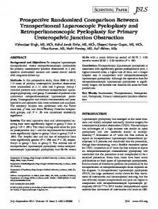
To examine the fundamental relationships between cover, cost, and overlap, Pareto fronts based on T est1 and T est2 were investigated. In these figures, the Pareto fronts using N S with seven α settings (i.e., α = 0,10,20,30,40,50,60) are displayed. Seven settings, instead of all 13, were used to improve the readability of the figures. Figures 8, 9, 10 display the Pareto fronts on T est1 for 45 km2 problem instances. The Pareto fronts indicate that as the α setting increases (and the constraint is relaxed), higher service coverage is obtained–but at the expense of increasing cost. Also, as the candidate site density increases, the demarcation between solutions improves. This suggests, for example, that higher density cell plans show performance differences more markedly. Pareto Plot: 45 x 45 x 61 (v1)
55 50 45
Cost in Units
40
improves. However, this was even more marked on T est2 . More importantly, these figures show that total cell overlap can be controlled effectively by altering the α setting of the decoder.
45 40 35 30
0% 10% 20% 30% 40% 50% 60%
25 20 15 10 5 0 30
40
50
80
30
70
25 20 60
80
90
Pareto Plot: 45 x 45 x 122 (v1)
90
50
70
Figure 11: Pareto plot: T est2 , 45 km2 with 61 sites
0% 10% 20% 30% 40% 50% 60%
40
60
% Service Coverage
35
15 30
Pareto Plot: 45 x 45 x 61 (v1)
50
% Overlap
Examine Pareto fronts
% of Overlap in Cell Plans
3.3.3
70
80
90
% Service Coverage
60
0% 10% 20% 30% 40% 50% 60%
50 40 30 20 10
Figure 8: Pareto plot: T est1 , 45 km2 with 61 sites
0 50
60
70
80
90
100
Service Coverage
80 70
Cost in Units
60
Pareto Plot: 45 x 45 x 122 (v1)
Figure 12: Pareto plot: T est2 , 45 km2 with 122 sites
0% 10% 20% 30% 40% 50% 60%
50
100
40
% Overlap
80
30 20 50
Pareto Plot: 45 x 45 x 244 (v1)
120
60
70
80
90
Service Coverage
100
0% 10% 20% 30% 40% 50% 60%
60 40 20
Figure 9: Pareto plot: T est1 , 45 km2 with 122 sites
0 65
70
75
80
85
90
95
100
% Service Coverage Pareto Plot: 45 x 45 x 244 (v1)
90 80
Cost in Units
70 60
Figure 13: Pareto plot: T est2 , 45 km2 with 244 sites
0% 10% 20% 30% 40% 50% 60%
50 40 30 20 65
70
75
80
85
90
95
100
% Service Coverage
In summary, the Pareto figures show the fundamental relationships between the three objectives: (1) higher service coverage involves increasingly higher cost and (2) higher service coverage involves increasingly higher cell overlap. In terms of the overlap constraint, α = 35% results in the best performance in terms of coverage and cost, which suggests that the per unit cost of service coverage at this setting is lower than at any other setting.
Figure 10: Pareto plot: T est1 , 45 km2 with 244 sites
4.
Figures 11, 12, 13 display the Pareto fronts on T est2 for 45 km2 problem instances. As was seen in the T est1 , as the site density increases, the demarcation between solutions
In this paper, we have investigated the performance of a two-phase strategy to optimize base station site selection. Advantages of this strategy are (1) a range of high quality solutions are created reflecting trade-offs between multiple
CONCLUSIONS AND FUTURE WORK
objectives; (2) the computational complexity compared to an exhaustive search is reduced; (3) the abstract model increases flexibility and allows the use of the best and most recent multi-objective algorithms; and, (4) the relationships between objectives can be clearly seen when Pareto fronts are graphed.
5. REFERENCES [1] S.M. Allen, S. Hurley, and R.M. Whitaker. Automated decision technology for network design in cellular communication systems. In 35th International Conference on System Sciences, pages 1–8, 2002. [2] E. Amaldi, A. Capone, and F. Malucelli. Optimizing base station siting in UMTS networks. In Proceedings 53th IEEE Conference on Vehicular Technology, volume 4, pages 2828–2832, 2001. [3] R. Bose. A smart technique for determining base station locations in an urban environment. IEEE Journal on Selected Areas in Communications, 50(1):43–47, 2001. [4] K. Deb. Multi-Objective Optimization using Evolutionary Algorithms. John Wiley and Sons, 2001. [5] K. Deb, S. Agrawal, A. Pratap, and T. Meyarivan. A fast elitist non-dominated sorting genetic algorithm for multi-objective optimization: Nsga-ii. In Lecture Notes in Computer Science, volume 1917, pages 848–849, 2000. [6] K. Deb, L. Thiele, M. Laumanns, and E. Zitzler. Scalable test problems for evolutinary multi-objective optimization. In Kangal Report No. 2001001, pages 1–27, 2001. [7] E. Ekici and C. Ersoy. Multi-tier cellular network dimensioning. Wireless Networks, 7:401–411, 2001. [8] C.M. Fonseca and P.J. Fleming. On the performance assessment and comparison of stochastic multiobjective optimizers. In Fourth International Conference on Parallel Problem Solving from Nature, pages 584–593, 1996. [9] M. Galota, C. Glaßer, S. Reith, and H. Vollmer. A polynomial-time approximation scheme for base station positioning in UMTS networks. In 5th Discrete Algorithms and Methods for Mobile Computing and Communications Conference, pages 52–59, 2000. [10] J.K. Han, B.S. Park, Y.S. Choi, and H.K. Park. Genetic approach with a new representation base station placement in mobile communications. In Proceedings 54th IEEE Conference on Vehicular Technology, volume 4, pages 2703–2707, 2001. [11] Q. Hao, B. Soong, E. Gunawan, J. Ong, C.B. Soh, and Z. Li. A low-cost cellular mobile communication system: A hierarchical optimization network resource planning approach. IEEE Journal on Selected Areas in Communications, 15(7):1315–1326, 1997. [12] M. Hata. Empirical formula for propogation loss in land mobile radio services. IEEE Transactions on Vehicular Technology, 29(3):317–325, August 1980. [13] X. Huang, U. Behr, and W. Wiesbeck. Automatic base station placement and dimensioning for mobile network planning. In IEEE Vehicular Technology Conference, volume 4, pages 1544–1549, 2000. [14] X. Huang, U. Behr, and W. Wiesbeck. Automatic cell planning for a low-cost and spectrum efficient wireless
[15]
[16]
[17]
[18]
[19]
[20]
[21]
[22]
[23]
[24]
[25]
[26]
[27]
network. In Proceedings of Global Telecommunications Conference (GLOBECOM), volume 1, pages 276–282, 2000. S. Hurley and R.M. Whitaker. An agent based appraoch to site selection for wireless networks. In Symposium on Applied Computing, pages 1–4, 2002. V. Khare, X. Yao, and K. Deb. Performance scaling of multi-objective evolutionary algorithms. KanGAL Report No.2002009, pages 1–15, 2002. C.Y. Lee and H.G. Kang. Cell planning with capacity expansion in mobile communications: A tabu search approach. IEEE Transactions on Vehicular Technology, 49(5):1678–1691, 2000. R. Mathar and T. Neissen. Optimum positioning of base stations for cellular radio networks. Wireless Networks, 6:421–428, 2000. Herve Meunier, El-Ghazali Talbi, and Philippe Reininger. A multiobjective genetic algorithm for radio network optimization. In 2000 Congress on Evolutionary Computation, volume 1, pages 317–324, July 2000. L. Raisanen and R.M. Whitaker. Comparison and evaluation of multiobjective genetic algorithms for the antennae placement problem. To appear in Special issue of Monet: Algorithmic Solutions for Wireless, Mobile, and Ad Hoc Sensor Networks., pages 1–26, 2003. T. Starkweather, S. McDaniel, K. Mathias, D. Whitley, and C. Whitley. A comparison of genetic sequencing operators. In Rick Belew and Lashon Booker, editors, Proceedings of the Fourth International Conference on Genetic Algorithms, pages 69–76, San Mateo, CA, 1991. Morgan Kaufman. K. Tutschku. Interference minimization using automatic design of cellular communication networks. In IEEE Vehicular Technology Conference, pages 634–638, 1998. M. Vasquez and J-K. Hao. A heuristic approach for antenna positioning in cellular networks. Journal of Heuristics, 7:443–472, 2001. D.A. Veldhuizen and G.B. Lamont. On measuring multiobjective evolutionary algorithm performance. In Congress on Evolutionary Computation, pages 204–211, 2000. N. Weicker, G. Szabo, K. Weicker, and P. Widmayer. Evolutionary multiobjective optimization for base station transmitter placement with frequency assignment. IEEE Transactions on Evolutionary Computation, 7(2):189–203, 2003. E. Zitzler, M. Laumanns, L. Thiele, C. Fonseca, and G. da Fonseca. Performance assessment of multiobjective optimizers: An analysis and review. Technical Report 139, Computer Engineering and Networks Laboratory(TIK), ETH Zurich, Switzerland, 2002. E. Zitzler and L. Thiele. Multiobjective optimization using evolutionary algorithms–a comparative case study. In Parallel Problem Solving from Nature, pages 292–301, 1998.