A Comparison of Statistical Dynamical and Ensemble ... - AMS Journals

426

JOURNAL OF THE ATMOSPHERIC SCIENCES

VOLUME 65

A Comparison of Statistical Dynamical and Ensemble Prediction Methods during Blocking TERENCE J. O’KANE*

AND

JORGEN S. FREDERIKSEN

CSIRO Marine and Atmospheric Research, Aspendale, Australia (Manuscript received 25 September 2006, in final form 20 March 2007) ABSTRACT In this paper error growth is examined using a family of inhomogeneous statistical closure models based on the quasi-diagonal direct interaction approximation (QDIA), and the results are compared with those based on ensembles of direct numerical simulations using bred perturbations. The closure model herein includes contributions from non-Gaussian terms, is realizable, and conserves kinetic energy and enstrophy. Further, unlike previous approximations, such as those based on cumulant-discard (CD) and quasi-normal (QN) hypotheses (Epstein and Fleming), the QDIA closure is stable for long integration times and is valid for both strongly non-Gaussian and strongly inhomogeneous flows. The performance of a number of variants of the closure model, incorporating different approximations to the higher-order cumulants, is examined. The roles of non-Gaussian initial perturbations and small-scale noise in determining error growth are examined. The importance of the cumulative contribution of non-Gaussian terms to the evolved error tendency is demonstrated, as well as the role of the off-diagonal covariances in the growth of errors. Cumulative and instantaneous errors are quantified using kinetic energy spectra and a small-scale palinstrophy production measure, respectively. As a severe test of the methodology herein, synoptic situations during a rapid regime transition associated with the formation of a block over the Gulf of Alaska are considered. In general, the full QDIA closure results compare well with the statistics of direct numerical simulations.

1. Introduction The skill of numerical weather forecasts is determined by the instability properties of the atmospheric flow, analysis errors, and model deficiencies. Early attempts at establishing the theoretical limits to atmospheric predictability focused on error growth in deterministic forecasts, with the error determined from the divergence of pairs of initially close states (Charney 1966; Smagorinsky 1969; Kasahara 1972). However, it was realized that weather forecasting should be regarded either as a statistical problem of predicting the probability density function of atmospheric states or,

* Current affiliation: Centre for Australian Weather and Climate Research, Bureau of Meteorology, Melbourne, Australia.

Corresponding author address: Terence J. O’Kane, CAWCR, Bureau of Meteorology, 700 Collins St., Docklands 3008, Australia. E-mail: [email protected] DOI: 10.1175/2007JAS2300.1 © 2008 American Meteorological Society

JAS4104

equivalently, of calculating the moments of meteorological variables. The reasons that deterministic forecasts fail over reasonable prediction periods are in large part due to the inherent nonlinearity in the system and because of errors in the initial conditions that arise from the impracticality of observing the atmosphere in sufficient detail. In this paper, we compare predictions with a new inhomogeneous statistical closure model to the statistics of ensemble-averaged direct numerical simulations (DNS) in order to elucidate the role of non-Gaussian terms, for which some cumulants higher than second order are nonzero, in ensemble prediction studies. Our renormalized closure methodology is based on a representation of the two- and three-point cumulants as functionals of diagonal cumulant and response functions and is known as the quasi-diagonal direct interaction approximation (QDIA) (Frederiksen 1999). We also consider a regularized version of the QDIA (RQDIA) (O’Kane and Frederiksen 2004, hereafter OF2004), which includes the indirect interactions, and hence more complete non-Gaussian terms, through

FEBRUARY 2008

O’KANE AND FREDERIKSEN

modified interaction coefficients. We also consider the effects of off-diagonal covariances and non-Gaussian terms in the initial conditions. Finally, to touch upon the early works of Epstein (1969a,b) and Fleming (1971a,b), we consider the cumulant-discard (CD) approximation within the closure formulation in which third- and higher-order cumulants are discarded. By using the QDIA closure, and its variants, we have a methodology for quantifying the contributions of inhomogeneous perturbations and non-Gaussian terms to the evolution of error growth under varying approximations. Unlike previous closure (Leith 1971, 1974; Leith and Kraichnan 1972) and cumulant-discard (Epstein 1969a,b; Fleming 1971a,b; Epstein and Pitcher 1972; Pitcher 1977) approaches to ensemble prediction, we employ bred initial perturbations rather than random initial perturbations. Additionally, methods where cumulants higher than second order are discarded are known to suffer from a number of disadvantages, not least of which includes displaying negative energies and numerical instabilities. Higher-order cumulants have also been shown to be necessary to track regime transitions in low-dimensional (Miller et al. 1994) and atmospheric (T. J. O’Kane and J. S. Frederiksen 2007, unpublished manuscript) data assimilation studies. We show that they are of no less importance for the accurate determination of the predictability of atmospheric flows. Recent studies have suggested that for the relatively small (⬍100 realizations) ensemble sizes typically used in numerical weather prediction schemes there is little capacity to produce anything more than Gaussian statistics (Denholm-Price 2003). Additionally, novel information theoretic approaches are currently being applied to try to estimate the role of non-Gaussian terms in the predictability of large-scale barotropic flows (Kleeman and Majda 2005). Epstein (1969a,b) developed statistical dynamical prognostic equations based on a third- and higher-order cumulant-discard hypothesis to enable the direct forecasting of mean and variance information. Epstein called this approach stochastic dynamic prediction; it proved, however, to be impractical for large numbers of degrees of freedom. Subsequently, more satisfactory methods based on the application of homogeneous closure models were developed to estimate the theoretical skill of Monte Carlo (MC) forecasts (Leith 1971, 1974; Leith and Kraichnan 1972). Early ensemble prediction schemes with random initial perturbations were commonly referred to as Monte Carlo prediction in the literature. The performance of Epstein’s stochastic dynamic model, compared with that of MC and nonrealizable closure schemes, such as the quasi-normal (QN; Mil-

427

lionshtchikov 1941; Proudman and Reid 1954) and the eddy-damped quasi-normal (EDQN; Orszag 1970) closures, was studied in a low-resolution barotropic model by Fleming (1971a,b). Fleming found that the stochastic dynamic model was only valid for very short-range predictions of the order of a few days and that by ⬇13 days they deviated significantly from the Monte Carlo solution. In contrast, the EDQN, in which the higher-order cumulants are approximated by empirically damping the three-point non-Gaussian terms, was found to be in very close agreement with the MC solution out to 18 days. Pitcher (1977; Epstein and Pitcher 1972) subsequently applied the method of Epstein to study the growth of errors on simulated atmospheric flow patterns within an equivalent barotropic spectral model. Unfortunately, QN and EDQN closures may result in negative kinetic energies during such integrations; the EDQN needs to be Markovianized in order to be realizable. As noted above, Fleming (1971a,b) was the first to study predictability using nonrealizable non-Markovian closures based on the quasi-normal and eddy-damped quasi-normal hypotheses. The most well known of the subsequent realizable Markovianized versions is the eddy-damped quasi-normal Markovian model (EDQNM; Orszag 1970; Pouquet et al. 1975; Bowman et al. 1993), which has been widely applied to the study of the statistics of the predictability of homogeneous turbulent flows (Leith 1971; Métais and Lesieur 1986). A somewhat similar homogeneous statistical closure approach, known as the test field model (TFM), was also used by Leith (1974) and Leith and Kraichnan (1972) to examine error growth from isotropic initial conditions. Herring et al. (1973) examined error growth with a non-Markovian closure called the direct interaction approximation (DIA) and compared the DIA results with those of DNS in order to examine the predictability of decaying three-dimensional isotropic turbulence. The development of modern turbulence closures began with formulation of the second-order homogeneous direct interaction approximation by Kraichnan (1959). Closely related non-Markovian closures, such as Herring’s self-consistent field theory (SCFT; Herring 1965) and McComb’s local energy transfer theory (LET; McComb 1974; McComb and Shanmugasundaram 1984), are essentially variants of Kraichnan’s original DIA, which differ only in their application of the fluctuation dissipation theorem (Frederiksen and Davies 2000; Kiyani and McComb 2004). In the DIA the (direct) interactions between wavenumber components of the second-order cumulants and response functions are represented in terms of the same original (or “bare”)

428


interaction coefficients that appear in the DNS equations from which the closures are derived. Martin et al. (1973) showed that the formally exact statistical dynamical equations, including indirect interactions, require the modification (or “renormalization”) of the interaction coefficients (or “vertex functions”) that occur in the DIA approach. Frederiksen and Davies (2004) studied a regularized version of the DIA closure (RDIA) in which the interactions in wavenumber space are suitably localized through modified interaction coefficients. They found that the RDIA performed very accurately, both at the energy-containing large scales where the DIA also performs well, and as well at small scales where the DIA and related closures underestimate small-scale energy. Frederiksen and Davies (2004) review the physical foundation of the regularization method, including why it gives the correct inertial ranges consistent with the Kolmogorov hypotheses (Kraichnan 1964). This issue is further discussed in appendix C. The generalization of the DIA theory to formulate numerically tractable closures for inhomogeneous turbulence interacting with general mean flows has been an outstanding problem. Recently, Frederiksen (1999) developed the general QDIA theory and applied it to the interaction of two-dimensional inhomogeneous turbulence with general mean flows and topography. OF2004 implemented a computationally tractable cumulant update variant of the QDIA, including a generalized regularization methodology, in order to remove spurious nonlocal eddy-topographic and eddymean field interactions. The resulting RQDIA was found to perform very accurately at all scales with a computational cost only a few times larger than the RDIA. The QDIA closure has subsequently been generalized and implemented numerically to study the statistics of inhomogeneous turbulence interacting with general mean flows, topography, and Rossby waves on a generalized ␤ plane by Frederiksen and O’Kane (2005, hereafter FO2005). The QDIA is realizable and therefore does not become unstable for long run times, unlike the EDQN closures (Fleming 1971a). The QDIA is an improvement not just on the third-order cumulant-discard hypothesis, but also on empirically damped approximations to the higher-order cumulants. In common with all statistical dynamical methodologies, the QDIA model has no sampling error. It provides a clear-cut way of quantifying the relative importance of inhomogeneous perturbations and non-Gaussian terms. We apply it to show that there are essentially two regimes of error growth; first, when the errors are small, the tendency resulting from non-Gaussian effects is also small,

VOLUME 65

but their cumulative effects are still important, and second, when the errors saturate, non-Gaussian effects become increasingly important. In comparison to a single realization control forecast, ensemble forecasts are able to provide not only improved estimates of the mean, but also estimates of the forecast error variance and possibly the higher-order cumulants. In ensemble prediction schemes independent initial perturbations are generated as fast-growing disturbances with structures and growth rates typical of the analysis errors. In contrast, random initial perturbations sampled isotropically grow more slowly and are found to lead to underestimated error variances. This prompted Toth and Kalnay (1993) to develop a scheme in which initial forecast perturbations are generated through a breeding method. This method of bred perturbations allows information about the fast-growing errors to be incorporated into the initial perturbations for the forecast. For particularly dynamic flows, such as when emergent coherent structures are developing, errors arise due to fast-growing large-scale instabilities. Toth and Kalnay (1997) argue that the bred vectors are stochastically and nonlinearly modified versions of the leading Lyapunov vectors (LLVs); they also note that after an initial transient period (about a week or so), initial random perturbations growing on tropospheric flows converge on the structure of the LLVs (see also Frederiksen 2000). The perturbations are periodically rescaled using a global (or regional) scaling factor so that they approximate fast-growing errors within assimilation schemes. Tracton and Kalnay (1993) describe the implementation of an operational ensemble prediction scheme based on the breeding of growing modes. Houtekamer and Derome (1995) examined the relative performance of optimal perturbations, bred perturbations, and observational system simulation experiment perturbations for ensemble forecasts. Additionally, Houtekamer and Derome (1995) showed that the breeding method (Toth and Kalnay 1993, 1997; Frederiksen et al. 2004) is comparable to methods based on optimal perturbations or singular vectors (see Molteni et al. 1996; Frederiksen 2000) in terms of error reduction while being significantly easier to implement (Wei and Frederiksen 2004). It is on this basis and for simplicity and ease of implementation that we chose the breeding method. More recently, Wang and Bishop (2003) compared the breeding method to a methodology based on the ensemble transform Kalman filter, while Wei et al. (2006) recently implemented such an approach in an operational global prediction system. Many insights into atmospheric predictability have come from studies employing low-order models

FEBRUARY 2008

429


(Lorenz 1965; Anderson 1996), barotropic models (Frederiksen and Bell 1990; Molteni and Palmer 1993), and simplified and low vertical resolution baroclinic models (Farrell 1989; Frederiksen and Bell 1990; Molteni and Palmer 1993; Houtekamer and Derome 1995). In our present study, partly for simplicity and partly because we want to compare our results with those based on our recently developed closure model, we employ a barotropic model. We examine perturbation or “error” growth during a period in which a block started to form over the Gulf of Alaska around 5 November 1979. Therefore, our ensemble prediction study includes the regime transition from strongly zonal to blocked flow and samples the fast-growing instabilities associated with the development and maturation of a large-scale coherent structure. We have chosen to focus on the period between midOctober and mid-November 1979 over the Northern Hemisphere because blocking transitions are particularly difficult to predict (Frederiksen et al. 2004). The rapid growth of large-scale flow instabilities associated with the formation and decay of blocks leads to a corresponding rapid growth of the error covariance matrix. Thus, while our closure methodology is generally applicable to any atmospheric flow, the blocking transitions provide rigorous tests of the different closure variants that we employ. These regime transitions severely test the ability of the closure time history integrals to accurately capture the evolving covariances and higherorder non-Gaussian terms. Dynamical processes during blocking may have a baroclinic component, particularly in the early stages of development (Frederiksen 1983; Buizza and Molteni 1996; de Pondeca et al. 1998a,b), and this may be reflected in the error structures (Frederiksen and Bell 1990). However, a significant component of large-scale error growth can be described by barotropic dynamics, particularly during the more mature phase of blocking (Veyre 1991; Frederiksen 1998). Using both barotropic and baroclinic tangent linear models, Veyre (1991) showed that a large part of the error amplitude appears to be described by barotropic effects. The structure of this paper is as follows: In section 2 we briefly describe the spectral barotropic vorticity equation for flow over topography, including Rossby wave turbulence on a generalized ␤ plane and in the presence of a large-scale flow U. In section 3 we describe the cumulant closure problem and state the form of the QDIA closure equations with additional contributions from the off-diagonal covariance matrix and non-Gaussian terms at the initial time (OF2004; FO2005). Throughout this paper we use kinetic energy as a function of wavenumber as well as the palinstrophy

production measure as our main diagnostics; these are defined in section 4. In section 5 we outline our approach to ensemble prediction using the QDIA closure and variants. In particular, sections 5a and 5b outline the method of bred perturbations and the experimental design of our simulations. In section 6 ensemble prediction studies are performed in which comparisons are made between closure and ensemble-averaged DNS for error growth studies with a 5-day cycle during which bred perturbations are generated, followed by a 5-day forecast period. The fields in the numerical experiments are relaxed toward interpolated daily 500-mb observed streamfunction fields, starting on 26 October 1979 for the Northern Hemisphere. The discussion and conclusions are contained in section 7. Appendixes A, B, and C contain definitions of the interaction coefficients, closure equations, and regularization methodology, respectively.

2. Barotropic flow on a ␤ plane We base our studies of both ensemble prediction and the formulation of the statistical dynamical prediction equations on a generalized ␤-plane barotropic model for flow over topography. A more detailed exposition of the generalized ␤ plane and its conserved quantities, as well as the statistical mechanical equilibrium theory and nonlinear stability theory for flow on the generalized ␤ plane, can be found in FO2005. As noted there the full streamfunction is written in the form ⌿ ⫽ ␺ ⫺ Uy, where U is a large-scale east–west flow and ␺ represents the “small scales.” The evolution equation for the two-dimensional motion of the small scales over a mean topography is then described by the barotropic vorticity equation ⭸␨ ⫽ ⫺J共␺ ⫺ Uy, ␨ ⫹ h ⫹ ␤y ⫹ k 20Uy兲 ⫹ ␯ˆ ⵜ2␨ ⫹ f 0. ⭸t 共1a兲 Here f 0 is the forcing, ␯ˆ the viscosity, and J共␺, ␨兲 ⫽

⭸␺ ⭸␨ ⭸␺ ⭸␨ ⫺ ⭸x ⭸y ⭸y ⭸x

共1b兲

is the Jacobian. The vorticity is the Laplacian of the streamfunction ␨ ⫽ ⵜ2␺. The scale height for the topography h is given by h ⫽ (2␮gAH/RT0), where H is the height of the topography, R ⫽ 287 J kg⫺1 K⫺1 is the gas constant for air, T0 ⫽ 273 K is the horizontally averaged global surface temperature, g is the acceleration resulting from gravity, ␮ ⫽ sin(␾ ), ␾ is latitude, and A ⫽ 0.8 is the value of the vertical profile factor.

430


The term k 20Uy generalizes the standard ␤ plane by the inclusion of an effect corresponding to the solidbody rotation vorticity in spherical geometry where k0 is a wavenumber that specifies the strength of this large-scale vorticity. FO2005 noted that this additional small term results in a one-to-one correspondence between the dynamical equations, Rossby wave dispersion relations, nonlinear stability criteria, and canonical equilibrium theory on the generalized ␤ plane and the sphere. The barotropic vorticity equation and the form-drag equation for U can be made nondimensional by introducing suitable length and time scales, which we choose to be a/2, where a is the earth’s radius and ⍀⫺1 is the inverse of the earth’s angular velocity. With this scaling, we consider flow on the domain 0 ⱕ x ⱕ 2␲, 0 ⱕ y ⱕ 2␲. The form-drag equation for the large-scale flow U is the same as on the standard ␤ plane. With the inclusion of relaxation toward the state U it takes the form ⭸U 1 ⫽ ⭸t S

冕

h

S

⭸␺ dS ⫹ ␣共U ⫺ U兲. ⭸x

共2兲

Here, ␣ is a drag coefficient and S is the area of the surface 0 ⱕ x ⱕ 2␲, 0 ⱕ y ⱕ 2␲. In the absence of forcing and dissipation, Eqs. (1) and (2) together conserve kinetic energy and potential enstrophy. We derive the corresponding spectral space equations by representing each of the small-scale terms by a Fourier series; for example,

兺 ␨ 共t兲 exp共i k · x兲,

␨共x, t兲 ⫽

k

共3a兲

冋

VOLUME 65

册

⭸ ⫹ ␯0共k兲k2 ␨k共t兲 ⭸t ⫽

兺兺 ␦共k ⫹ p ⫹ q兲关K共k, p, q兲␨

⫺p␨⫺q

p∈T p∈T

⫹ A共k, p, q兲␨⫺ph⫺q兴 ⫹ f 0k ,

共4兲

where T ⫽ R ∪ 0 and the interaction coefficients are defined in appendix A. Here the complex ␯0(k) is related to the bare viscosity ␯ˆ and the intrinsic Rossby wave frequency ␻k by the expression

␯0共k兲k 2 ⫽ ␯ˆ k 2 ⫹ i␻k,

共5兲

where

␻k ⫽ ⫺

␤kx k2

共6兲

.

* and introduced We have defined ␨⫺0 ⫽ ik0U; ␨0 ⫽ ␨⫺0 a term h⫺0 that we take to be zero, but could more generally be related to a large-scale topography. We note that U is real and we have defined ␨0 to be imaginary. This is done to ensure that all of the interaction coefficients that we use are defined to be purely real. Also with ␨0 ⫽ ⫺ik0U, f 00 and ␯0(k0) are defined by f 00 ⫽ ␣␨0

共7兲

␯0共k0兲k 20 ⫽ ␣.

共8兲

These spectral equations are then the basis for our subsequent studies and theoretical developments. We can also consider the case where the bare forcing is replaced by a relaxation term of the form

k

⫺ ␨k兲, Sk共t兲 ⫽ ␬共␨ obs k

where

␨k共t兲 ⫽

1 共2␲兲2

冕

2␲

d2x ␨共x, t兲 exp共⫺i k · x兲,

共3b兲

where ␬ is the strength of the relaxation and linearly interpolated daily observed fields.

共9兲

␨ obs k

are

0

and x ⫽ (x, y), k ⫽ (kx, ky), k ⫽ (k 2x ⫹ k 2y)1/2 and ␨⫺k is conjugate to ␨k. As noted in Eq. (4.1) of FO2005, the sums in the consequent spectral equations run over the set R consisting of all points in discrete wavenumber space, except for point (0, 0). However, it was also observed that the form-drag equation for U can be written in the same form as that for the small scales by defining suitable interaction coefficients, representing the largescale flow as a component with zero wavenumber and extending the sums over wavenumbers. The spectral form of the barotropic vorticity equation with differential rotation, describing the evolution of the small scales, and the form-drag equation may then be written in the same compact form as for the f plane,

3. The closure equations The QDIA closure equations were derived by Frederiksen (1999) for general barotropic mean flows interacting with inhomogeneous turbulence over topography on an f plane. OF2004 tested the performance of the closure, including cumulant update and regularized variants, while the generalization to Rossby wave turbulence on a ␤ plane was formulated and tested by FO2005. Here we very briefly summarize the ␤ plane QDIA equations. We consider an ensemble of flows satisfying the generalized spectral barotropic vorticity equation [Eq. (4)] that describes the evolution of both the small and the large scales through the form-drag equation. Through-

FEBRUARY 2008

out this section the wave vectors range over the set T ⫽ R ∪ 0. We can express the vorticity ␨k and forcing f 0k in terms of their ensemble average means, denoted by 具典, and the deviations from the means, denoted by ˆ,

冋

册

⭸ ⫹ ␯0共k兲k 2 具␨k典 ⫽ ⭸t

冋

册

␨k ⫽ 具␨k典 ⫹ ␨ˆ k;

f 0k ⫽ 具f 0k典 ⫹ fˆ 0k.

共10兲

Then, the equation for the ensemble mean and perturbation fields can be written in the form

兺兺 ␦共k ⫹ p ⫹ q兲关K共k, p, q兲兵具␨

典具␨⫺q典 ⫹ C⫺p,⫺q共t, t兲其 ⫹ A共k, p, q兲具␨⫺p典h⫺q兴 ⫹ 具 f 0k典,

⫺p

p

q

共11兲

⭸ ⫹ ␯0共k兲k 2 ␨ˆ k ⫽ ⭸t

兺兺 ␦共k ⫹ p ⫹ q兲K共k, p, q兲关具␨

典␨ˆ ⫺q ⫹ ␨ˆ ⫺p具␨⫺q典 ⫹ ␨ˆ ⫺p␨ˆ ⫺q ⫺ C⫺p,⫺q共t, t兲兴

⫺p

p

⫹

q

兺兺 ␦共k ⫹ p ⫹ q兲A共k, p, q兲␨ˆ p

⫺ph⫺q

C⫺p,⫺q共t, s兲 ⫽ 具␨ˆ ⫺p共t兲␨ˆ ⫺q共s兲典,

共13兲

where p and q both range over the set T ⫽ R ∪ 0. Thus, we see from Eq. (11) that to determine the mean field we need an equation for the two-point cumulant C⫺p,⫺q(t, t). Multiplying Eq. (12) by ␨ˆ ⫺k(t⬘) and averaging leads to the following expressions for the diagonal two- and single-time cumulants in terms of two-

册

⭸ ⫹ ␯0共k兲k 2 Ck共t, t⬘兲 ⫽ ⭸t

⫹ fˆ 0k.

共12兲

q

Here the covariance matrix or two-point cumulant is defined by

冋

431


and three-point terms. Thus, the second-order cumulant requires knowledge of the third-order cumulant, which in turn depends on the fourth, and so on. We are consequently faced with two problems, namely, the cost of computing the full covariance matrix, which is prohibitive at any reasonable resolution (Kraichnan 1972), and second, the closure problem. By multiplying Eq. (12) by the conjugate term ␨ˆ ⫺k(t⬘), we obtain the expression for the diagonal twotime two-point cumulant in terms of the two- and threepoint cumulants,

兺兺 ␦共k ⫹ p ⫹ q兲A共k, p, q兲C

⫺p,⫺k共t,

p

t⬘兲h⫺q ⫹

q

兺兺 ␦共k ⫹ p ⫹ q兲K共k, p, q兲 p

q

⫻ 关具␨⫺p共t兲典C⫺q,⫺k共t, t⬘兲 ⫹ C⫺p,⫺k共t, t⬘兲具␨⫺q共t兲典 ⫹ 具␨ˆ ⫺p共t兲␨ˆ ⫺q共t兲␨ˆ ⫺k共t⬘兲典兴 ⫹ 具 fˆ 0k共t兲␨ˆ ⫺k共t⬘兲典 ⫽ Nk共t, t⬘兲, where we have used the abbreviation Ck(t, t⬘) ⫽ Ck,⫺k(t, t⬘). It is also convenient to separate the enstrophy production into the contributions from the two(inhomogeneous) and three-point (non-Gaussian) terms, Nk共t, t⬘兲 ⫽ N Ik共t, t⬘兲 ⫹ N Sk共t, t⬘兲, N Ik共t, t⬘兲 ⫽

兺兺 p

⫹

兺兺 ␦共k ⫹ p ⫹ q兲K共k, p, q兲 q

共16兲


冋

␦共k ⫹ p ⫹ q兲A共k, p, q兲C⫺p,⫺k共t, t⬘兲h⫺q

⫻ 关具␨⫺p共t兲典C⫺q,⫺k共t, t⬘兲 ⫹ C⫺p,⫺k共t, t⬘兲具␨⫺q共t兲典兴,

N Sk共t, t⬘兲 ⫽

where 具fˆ 0k(t)␨ˆ ⫺k(t⬘)典 is a stochastic forcing term, defined by Eq. (B7) of appendix B, and F 0k(t, s) ⫽ 具fˆ 0k(t)fˆ 0* k (s)典 is the variance of the random forcing fˆ 0k. The equation for the diagonal single-time cumulant is

共15兲

q

p

共14兲

q

⫻ 具␨ˆ ⫺p共t兲␨ˆ ⫺q共t兲␨ˆ ⫺k共t⬘兲典 ⫹ 具 fˆ 0k共t兲␨ˆ ⫺k共t⬘兲典,

共17兲

册

⭸ ⫹ 2ℜ␯0共k兲k 2 Ck共t, t兲 ⫽ 2ℜNk共t, t兲. ⭸t

共18兲

For Eqs. (11), (14), and (18) to form a closed system of statistical closure equations, we need to express C⫺p,⫺q (t, t⬘) and 具␨ˆ ⫺p(t)␨ˆ ⫺q(t)␨ˆ ⫺k(t⬘)典 in terms of the mean field 具␨ˆ (t)典 and the diagonal cumulant C (t, t⬘). k

k

To this end a statistical closure methodology based on a QDIA (Frederiksen 1999; OF2004; FO2005) is employed. The QDIA closure makes the replacements ˆ ˆ ˆ C⫺p,⫺q(t, t⬘) → CQDIA ⫺p,⫺q(t, t⬘) and 具␨⫺p(t)␨⫺q(t)␨⫺k(t⬘)典 → 具␨ˆ (t)␨ˆ (t)␨ˆ (t⬘)典QDIA, which are functionals in ⫺p

⫺q

⫺k

terms of the mean field, topography, and diagonal cu-

432


mulant and response functions defined in Eqs. (B8)– (B10) of appendix B, respectively.

VOLUME 65

Then, the palinstrophy production measure P M can be defined in terms of these quantities by P M共t兲 ⫽ 2K Ⲑ共PˆFˆ 1Ⲑ2兲,

4. Diagnostics Next, we define a number of diagnostics that we employ in the following section for analyzing the predictability studies. We define the perturbation (error) eT(kx, t) and mean eM(kx, t) kinetic energy spectra as functions of zonal wavenumber by eT共kx , t兲 ⫽ e M共kx , t兲 ⫽

1 2

兺

1 2

兺关具␨ 共t兲典具␨

关Ck共t, t兲兴 Ⲑk 2,

共19a兲

Pˆ 共t兲 ⫽

⫽I K共t兲 ⫹ S K共t兲,

共26兲

where I K共t兲 ⫽ 2K IⲐ共PˆFˆ 1Ⲑ2兲,

共27兲

S K共t兲 ⫽ 2K SⲐ共PˆFˆ 1Ⲑ2兲.

共28兲

ky

典兴 Ⲑk 2.

⫺k共t 兲

k

共19b兲

ky

The kinetic energy of the large-scale flow is plotted at kx ⫽ 0. We shall also use a measure based on palinstrophy production to characterize the small-scale error growth during forecasts. For this it is useful to separate the enstrophy production terms as in Eq. (15) into the contribution from the two-point inhomogeneous N I(t, t), and three-point non-Gaussian N S(t, t), terms. The palinstrophy production measure based on the three-point non-Gaussian terms is just the skewness S K that has been commonly used to examine the small-scale behavior of homogeneous (Herring et al. 1974; Frederiksen and Davies 2000) and inhomogeneous turbulence (OF2004). The current regime of small-amplitude transient errors growing on larger-amplitude mean flows, however, differs from these previous studies, in that most of the transfer results from the two-point inhomogeneous production. One of our aims will be to quantify the relative contribution of the two-point and nonGaussian terms to both the instantaneous and cumulative error growth. Examination of both the palinstrophy production and kinetic energy spectra allows this quantification. We begin by specifying the perturbation enstrophy Fˆ, perturbation palinstrophy Pˆ, and palinstrophy production K by Fˆ 共t兲 ⫽

共25兲

1 2

兺 C 共t, t兲,

1 2

兺 C 共t, t兲k ,

共20兲

k

k

2

k

K 共t兲 ⫽ K I共t兲 ⫹ K S共t兲,

兺 k t兲, 共t兲 ⫽ 兺 k N 共t, t兲.

K 共t兲 ⫽ I

共21兲

k

2

共22兲

N Ik共t,

共23兲

S k

共24兲

5. Blocking, breeding, and experimental design In the studies that follow we focus on the ensemble predictability of 500-hPa Northern Hemisphere atmospheric flows during a period in October and November 1979, in which a large-scale blocking high–low dipole formed over the Gulf of Alaska on 5 November, amplified and persisted until 12 November, and then weakened and moved downstream. This period has been recently examined by Frederiksen et al. (2004) using two different general circulation models (GCMs), with a breeding scheme to generate initial perturbations. Our aim is to compare closure and ensembleaveraged DNS results for 5-day forecasts starting after a 5-day breeding period using the closure to separate and quantify the various contributions to error organization and growth. The DNS is used as a measure of the accuracy of the closure. The formation (and decay) of large-scale blocking high–low dipoles associated with the transition from strongly zonal to blocked (and blocked to zonal) flow correspond to periods of decreased predictability.

a. Bred initial forecast errors In order for the initial perturbations in our error growth (forecast) experiments to capture the fastgrowing instabilities of the day, we employ the method of bred perturbations developed by Toth and Kalnay (1993). We start the breeding cycle from an initially Gaussian isotropic error field and take a continuous approach to breeding in which the evolving perturbation is scaled after every time step. The global scaling parameter is defined in terms of the streamfunction, because for atmospheric flows it is the large scales that are of primary importance in determining the dynamics, and hence error growth. The global scaling factor for adjusting the perturbation field is defined as

k

KS

2

k

g共t兲 ⫽

冋

⌺kCk共t0, t0兲 Ⲑk 4 ⌺kCk共t, t兲 Ⲑk 4

册

1Ⲑ2

,

共29a兲

FEBRUARY 2008


and the scaling is performed as follows:

␨ˆ k共t⫹兲 ⫽ g共t兲␨ˆ k共t⫺兲,

共29b兲

Ck共t⫹, t⫹兲 ⫽ g共t兲g共t兲Ck共t⫺, t⫺兲,

共29c兲

Ck共t⫹, t⬘⫹兲 ⫽ g共t兲g共t⬘兲Ck共t⫺, t⬘⫺兲,

共29d兲

where ⫺ and ⫹ indicate prior and posterior fields, respectively. In both the DNS and closure the offdiagonal elements of the covariances are adjusted. In the DNS this occurs through direct application of the global scaling factor to the vorticity field [Eq. (29b)], whereas in the closure it occurs through the diagonal cumulant that in turn scales the off-diagonal elements through Eq. (B8) of appendix B. Prior to breeding, isotropic initial perturbations have no structural organization. After the breeding period the initial forecast error fields are organized so that they contain information about the fast-growing errors (incorporated during the breeding cycle) arising because of instabilities present in the underlying dynamics of the flow (Toth and Kalnay 1993, 1997).

b. Experimental design We examine the evolution of transient error fields in closure and DNS calculations on trajectories similar to that taken by the atmospheric 500-hPa field between 26 October and 8 November 1979. For the mean fields within a barotropic model to closely follow an observed trajectory, it is necessary to specify suitable timeevolving source terms. A relaxation term of the form Sk共t兲 ⫽ ␬共␨ obs ⫺ ␨k兲 k

共30兲

is added to the right-hand side of the spectral barotrois the linearly interpic vorticity equation, where ␨ obs k polated daily observed 500-hPa streamfunction fields at 1200 UTC. We generate a truth trajectory beginning on 26 October 1979 by running the barotropic model with a relaxation term [Eq. (30)] interpolating down to the required time step and use an e-folding relaxation time of 2 days. The source term is calculated at each time step of the unperturbed truth simulation, stored, and then applied to both perturbed ensemble DNS runs and the mean field equation of the closure. This ensures that the truth field closely follows the observed trajectory, but that the perturbations are not additionally damped as further discussed by FO2005. We present results for k 20 ⫽ 1⁄2 and ␤ ⫽ 1⁄2 (a dimensional value of 1.15 ⫻ 10⫺11 m⫺1 s⫺1) typical of the ␤ effect at 60° latitude. Throughout we employ a viscosity of 2.5 ⫻ 105 m2 s⫺1 corresponding to a nondimensional value of ␯ˆ ⫽ 3.378 ⫻ 10⫺4. Both closure and DNS are

433

run with a 1-h time step. In all calculations we use a circular truncation in wavenumber space with a maximum wavenumber of k ⫽ 16 (C16). The initial errors fields are taken to be Gaussian distributed with isotropic kinetic energy spectra that are approximately constant with wavenumber (apart from the zero component). Such flat spectra are reasonably consistent with atmospheric error fields (Molteni et al. 1996; Wei and Frederiksen 2004). In all of the calculations that follow, the initial perturbations, or errors, prior to breeding are Gaussian and isotropic and are several orders of magnitude less than the mean field at all wavenumbers. We again take the approach of FO2005, where the initial DNS fields are constructed by first taking a Gaussian sample with zero mean and unit variance, and then for a given realization obtaining further members of the ensemble by moving its origin by an increment in the x direction and then in the y direction. The initial realization is moved successively by 2␲/n in the x direction to form n realizations. Each of these n realizations is then shifted by 2␲/n in the y direction to form a total of n2 realizations. To guarantee minimal sampling errors we then take the negative value of each of the n2 elements; thus, we now have an ensemble of 2n2 realizations. The same process is then repeated with further initial Gaussian samples until an ensemble of the required number is obtained. This method ensures that not only are the initial fields prior to breeding accurate, but that the initial DNS covariance matrix is effectively isotropic for large enough n. For the DNS we show that the ensemble average results from 1800 simulations, although we found comparable results for 32 realizations, which is in agreement with the findings of Leith (1974) and Houtekamer and Derome (1995). In the studies that follow the closure variants were implemented with a single restart or cumulant update at day 5. The RQDIA, zeroed RQDIA (ZRQDIA), and CD calculations are regularized in the manner of OF2004. The regularization procedure localizes the interactions by modifying the interaction coefficients K(k, p, q) and A(k, p, q) in the two-time cumulant and response function equations of the QDIA closure (see appendix C).

6. Ensemble prediction results Data assimilation studies of low-order, strongly nonlinear flows, such as the Lorenz equations (Miller et al. 1994), have shown that third-order and higher cumulants are required in order to track regime transitions. More recently, T. J. O’Kane and J. S. Frederiksen (2007, unpublished manuscript) have also shown the

434


importance of these non-Gaussian terms in data assimilation studies using barotropic models during block formation, maturation, and decay. We now compare DNS and closure experiments using bred initial ensemble perturbations in an examination of ensemble prediction during blocking. In this section we investigate the role of nonGaussian terms in error growth during block formation and maturation by comparing the performance of the QDIA closure and variants to DNS. The QDIA includes only direct interactions in the equations describing the two- and three-point cumulants. In the regularized QDIA, the indirect interactions are represented through modified interaction coefficients that localize interactions in wavenumber space; this yields improved spectra and estimates of non-Gaussian terms. Comparison of the QDIA and RQDIA closures elucidates the role of improved higher-order approximations to nonGaussian terms on error growth. Both the QDIA and RQDIA include non-Gaussian initial forecast perturbations at the close of the breeding cycle through the cumulant-update restart procedure (OF2004). A further closure variant (ZRQDIA) enables the forecast to be initialized with the same variances as the RQDIA, but with homogeneous rather than inhomogeneous and non-Gaussian initial perturbations. We compare the ZRQDIA and RQDIA closures to determine the role of initial off-diagonal covariances and non-Gaussian terms on error growth. Comparison of the evolved kinetic energy for DNS and the various closures allows us to investigate the cumulative contributions of nonGaussian terms to error growth. We additionally use the palinstrophy production measure P M ⫽ I K ⫹ SK (defined in section 4) to quantify instantaneous contributions from non-Gaussian (three-point tendencies) and off-diagonal (two-point tendencies) terms. We also examine the performance of a CD approximation, in which the three-point and higher-order cumulants are discarded in the closure. This then makes direct connection with previous work discussed in the introduction and allows us to examine the contribution to error growth resulting from second-order cumulants only. Throughout our studies, DNS results for large ensemble sizes (ⱖ1800 realizations) are taken as the benchmark. Each of these different closure variants elucidates the role of processes that contribute to error growth. These processes may be associated either with flow inhomogeneities and the rapid growth of offdiagonal covariances or from the accumulated contributions of the higher-order non-Gaussian terms. A summary of the properties of the different closure models is given in Table 1.

VOLUME 65

TABLE 1. Summary of the different closure variants. QDIA

Direct interactions only Inhomogeneous ⫹ non-Gaussian initial forecast perturbations RQDIA Direct ⫹ indirect interactions Inhomogeneous ⫹ non-Gaussian initial forecast perturbations ZRQDIA Same as for RQDIA, but with homogeneous initial forecast perturbations No initial information from off-diagonal covariances or non-Gaussian terms at time of forecast CD Same as for RQDIA, but with third cumulant discard

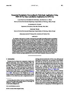
a. Comparison of breeding in RQDIA, QDIA, and DNS In Fig. 1 we compare the DNS, QDIA, and RQDIA calculations, starting with 5-day breeding cycles on 26 October 1979 with isotropic initial perturbations (Fig. 1a). After the 5-day breeding period (Fig. 1b) we show that the mean kinetic energies as functions of zonal wavenumber for all three calculations are in good agreement, but that the QDIA perturbation energy is slightly underestimated at the small scales compared with the RQDIA results. The bred perturbations are clearly peaked at k ⫽ 3, which is the dominant wavenumber of the fastest-growing mode. Figure 1c shows the results after a subsequent 5-day forecast period, where it is evident that the error field is saturating at the small scales. RQDIA is, in general, in close agreement with DNS, while QDIA slightly underpredicts the evolved small-scale error energy. The reason for the underestimation of small-scale energy with the QDIA closure is due to the neglect of indirect interactions as discussed in the introduction and appendix C. We next employ the palinstrophy production measure, which is defined in section 4 as a sensitive measure of the small-scale differences between closure variants and DNS. We see from the palinstrophy production measure in Fig. 1d that there are four distinct regimes in the organization and growth of errors during the depicted 10-day experiment. The first two regimes corresponding to the organization and formation of error structures are contained within the 5-day breeding period starting on 26 October 1979. During the first day of breeding there is a dramatic and rapid growth in the palinstrophy production measure, associated with the growth of the off-diagonal covariances and the organization of error structures. As the initial error field evolves and organizes from Gaussian isotropic initial perturbations, with error variances rescaled by the breeding factor [Eqs. (29)], P M grows to values determined largely by flow inhomogeneities. From approxi-

FEBRUARY 2008


435

FIG. 1. Bred perturbations are generated over a 5-day period starting on 26 Oct 1979, followed by a 5-day forecast period. The initial, day-5, and day-10 mean and perturbation kinetic energy (nondimensional) as functions of zonal wavenumber are shown for (a) DNS, (b) QDIA, and (c) RQDIA calculations. (d) The DNS, QDIA, and RQDIA palinstrophy production measure over the entire 10-day period are also shown.

mately day 2 through to day 5, the palinstrophy production measure P M continues to grow, although now at a significantly reduced rate. The final two regimes occur during the forecast period and correspond to rapid growth and the eventual saturation of errors. At day 5 the breeding ends, the restart procedure is implemented, and the forecast begins with flow-dependent initial perturbations. The error fields, with structures of the leading instability vectors, now amplify rapidly, and this is associated with an accompanying drop in the palinstrophy production measure. The rapid rate of error growth postbreeding is reflected in the overall downward slope of the palin-

strophy production measure during this period. The drop in the palinstrophy is due to the growth of the instability vectors at the large scales (cf. Frederiksen et al. 1996). From day 7 onward, the growth of the error field is much reduced as the error starts to saturate at about day 10. During the period in which the error kinetic energy is growing the evolution of P M is largely determined by the dynamics of the large-scale flow instabilities. In this regime, P M ⬇ I K. It is only as the errors start to saturate that non-Gaussian terms begin to become increasingly important. In the freely decaying homogeneous turbulence studies of Herring et al. (1974) and Frederiksen and Davies (2000), P M ⫽ SK

436


VOLUME 65

FIG. 2. Bred perturbations are generated over a 5-day period starting on 27 Oct 1979, followed by a 5-day forecast period. The (a) initial, (b) day-5, and (c) day-10 mean and perturbation kinetic energy (nondimensional) as functions of zonal wavenumber are shown. (d) The DNS and closure palinstrophy production measure over the entire 10-day period are also shown.

and saturates at a nearly constant value. The inhomogeneous turbulence studies of OF2004 further showed that as resolution increases the contribution resulting from the non-Gaussian terms becomes correspondingly more important, dominating at the small scales for typical atmospheric spectra. In Figs. 2 and 3 we compare DNS to RQDIA starting on 27 and 28 October, respectively, and find similar agreement in the day-5 and day-10 zonally averaged kinetic energy to that observed in Fig. 1. In addition, we again see similar behavior to that in Fig. 1d for the evolving P M, with the four regimes discussed previously again evident in Figs. 2d and 3d; the RQDIA closure compares very well with ensemble-averaged DNS (1800 realizations) in all cases. The results in Figs. 1–3, including the very close agreement between closure and DNS,

are typical of our more extensive studies (not shown) and demonstrate the robustness of our findings. That RQDIA and DNS are in such close agreement demonstrates the importance of the missing indirect interactions in the QDIA closure, indicating that all higher-order moments must be accurately accounted for. At low to moderate resolution, the moments coupling eddies to both the topography and mean field are most critical to accurate error covariance estimation. However, the cumulative contribution from the evolving higher-order non-Gaussian terms is still required in order to achieve close comparison with DNS.

b. The role of non-Gaussian terms in error growth We next compare the behavior of the different versions of the QDIA closure with that of DNS over a

FEBRUARY 2008


437

FIG. 3. Bred perturbations are generated over a 5-day period starting on the 28 Oct 1979, followed by a 5-day forecast period. The (a) initial, (b) day-5, and (c) day-10 mean and perturbation (nondimensional) kinetic energy as functions of zonal wavenumber are shown. (d) The DNS and closure palinstrophy production measure over the entire 10-day period are also shown.

10-day period, comprising 5 days of breeding followed by a 5-day forecast beginning on 29 October 1979. The evolved mean and perturbation kinetic energy as functions of zonal wavenumber are shown in Fig. 4. The RQDIA and ZRQDIA closures include both direct and indirect interactions, whereas QDIA has direct interactions only. Both the QDIA and RQDIA begin the forecast period with non-Gaussian initial perturbations, whereas ZRQDIA uses homogeneous initial perturbations. Specifically, ZRQDIA is identical to RQDIA; however, ZRQDIA begins the forecast period with all earlier contributions from the time history integrals omitted. Thus, ZRQDIA contains no initial information about the off-diagonal two- and three-point cumu-

lants; however, it uses the same bred initial diagonal two-point functions as RQDIA. We note from Fig. 4 that RQDIA and DNS are in good agreement at most scales, apart from some overestimation of the RQDIA transients at wavenumber kx ⫽ 1. QDIA is in good agreement with RQDIA and DNS at the large scales with k ⬍ 7, but falls away, underpredicting the small-scale perturbation kinetic energy. The performance of the ZRQDIA closure with the two- and three-point restart terms zeroed in Fig. 4 dramatically demonstrates the effect of purely homogeneous initial perturbations in suppressing the rate at which the error kinetic energy grows; we see that ZRQDIA systematically underpredicts the evolved

438


VOLUME 65

FIG. 4. (a) Mean and (b) transient kinetic energy (nondimensional) as functions of zonal wavenumber after 5 days breeding and 5 days forecast on 8 Nov for RQDIA, QDIA, ZRQDIA, and DNS calculations. The mean spectra are nearly indistinguishable for all models.

day-10 error kinetic energy at all scales. This underprediction occurs because ZRQDIA removes all information contained in the time history integrals and restarts the closure calculation at day 5, with no initial contributions from off-diagonal covariances or from nonGaussian terms. The initial error field only includes the homogeneous contribution. Any information about the off-diagonal inhomogeneities and non-Gaussian terms accumulated in the time history integrals has been removed. The results in Fig. 4 demonstrate the importance of the cumulative contribution of higher-order indirect interactions (RQDIA) and initial off-diagonal covariances and non-Gaussian terms to the evolved small-scale perturbation kinetic energy. In Fig. 5a we compare the small-scale differences between the different closures and DNS. We compare the results of using homogeneous initial forecast perturbations within the ZRQDIA closure with those for bred perturbations, including off-diagonal covariance and non-Gaussian contributions within the RQDIA closure, and for DNS. We find that after the restart P M grows very rapidly within the ZRQDIA closure as the off-diagonal covariances develop. The results for RQDIA and DNS are in broad agreement, whereas the decay of P M for ZRQDIA consistently lags that of RQDIA during the forecast. The use of homogeneous initial forecast errors, that is, diagonal error variances, discards flow-dependent correlations (off-diagonal covariances), leading to the systematic underestimation of

both large- and small-scale forecast errors. In Fig. 5a we see that ZRQDIA on day 5 (3 November 1979) must rebuild all off-diagonal covariances in order for error growth to occur (see also Toth and Kalnay 1993). The growth of off-diagonal covariances from isotropic initial perturbations was found to typically occur on the order of 1 day during the formation of this particular block. In Fig. 5b we quantify the relative contributions from SK and I K to P M at each time step. An important result in Fig. 5b is that at any given time the three-point contribution to the palinstrophy measure is less than 1% and that the growth of the error field is completely dominated by the two-point contribution. This makes sense because we are in a regime that is dominated by eddy–mean field and eddy–topographic interactions, and it is not until the error field saturates at the amplitude of the mean that we can begin to see an increase in the importance of contributions from the three-point (eddy–eddy) terms. For cases without breeding, such as for evolution from isotropic initial perturbations, the saturation times were found to be approximately 10 days, compared to the 5 days needed for breeding. In these cases the fact that the perturbation amplitudes were able to dominate the mean amplitudes at most scales resulted in much larger values for SK (up to ⬇20%) on day 10. As expected, the comparison of ZRQDIA with RQDIA clearly demonstrates that to neglect the contributions of the two- and three-point time history

FEBRUARY 2008


FIG. 5. (a) The P M(t) for 29 Oct–8 Nov 1979 for both RQDIA and ZRQDIA, and (b) P M(t), SK(t), and I K(t) for the same period for both the RQDIA and QDIA are shown. In (b), P M(t) and I K(t) are nearly equal for both the RQDIA and ZRQDIA, respectively.

terms is to reduce the rate of growth of the perturbation or error field. In Fig. 4 we saw that the evolved error fields on 8 November 1979 clearly show ZRQDIA and QDIA underestimating the evolved error energy amplitudes, while the RQDIA results compare closely to DNS. Importantly, even though the instantaneous nonGaussian terms in Fig. 5b may be small, they have an appreciable cumulative contribution to error growth. Figure 6a further illustrates the role of non-Gaussian terms; it shows the evolution of the ratio of the evolved perturbation to mean field over the 10-day period. In Fig. 6b we show the corresponding evolved error kinetic energy as a function of zonal wavenumber for ZRQDIA, RQDIA, and DNS. In Fig. 6a, the evolved ratios are plotted at 2.5-day intervals and are scaled by factors of 10, so as to be separated, and therefore visible on the same plot. ZRQDIA and RQDIA are identical

439

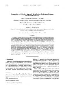
up to the end of the breeding period at day 5. At day 7.5 RQDIA, as expected, outperforms ZRQDIA. We take saturation to occur when the perturbation kinetic enˆ (t) is approximately equal to the mean kinetic ergy E k energy 具Ek典 over most scales, which, as shown in Fig. 6a, occurs at approximately day 5 of the forecast period. Once saturation occurs error growth slows dramatically and the evolved ZRQDIA kinetic energy is able to catch up to RQDIA and DNS. This picture is repeated in the evolution of the kinetic error energy depicted in Fig. 6b. In contrast to bred perturbations, random initial errors sampled isotropically grow much more slowly, as noted by Toth and Kalnay (1993), reaching saturation in 10 days. In Fig. 6c we compare the evolution of total kinetic energy over the 10-day period. We see close agreement between DNS and the closure variants throughout the initial 5-day breeding cycle, followed by some underestimation of total kinetic energy by ZRQDIA, and less so for RQDIA, after a subsequent 5-day forecast period. The results of Fig. 6c extend the closure study of error energy for decaying isotropic turbulence made by Herring et al. (1973; Fig. 2) to inhomogeneous flows using the direct interaction approximation formulated for difference velocity fields and compared with DNS results. In Fig. 7, for the case considered previously in Figs. 4–6, we see the very close agreement between DNS and RQDIA in the large scales of the zonally asymmetric or eddy streamfunction (pattern correlations typically of 0.9) over the entire 10-day period. We can also clearly see the high–low blocking dipole forming over the Gulf of Alaska on 8 November 1979. In our ensemble prediction studies there is the potential, given sufficient time, for the bred perturbations to converge onto Lyapunov vector 1 as a result of breeding using a global scaling factor. Bred vectors are superpositions of the local time-dependent LLVs of the flow (Toth and Kalnay 1997), and after an initial transient period (⬇7 days for atmospheric flows) all random perturbations assume the structure of the LLVs. We have repeated the experiment starting on 29 October with an additional stochastic backscatter forcing of the small scales. The stochastic backscatter forcing (Fig. 8d) corresponds to an injection of energy from the subgrid-scale eddies to the retained scale eddies, thereby randomly forcing the small-scale perturbations. The form chosen is similar to that calculated by Frederiksen and Davies (1997) using the EDQNM closure model. The stochastic backscatter has isotropic variance Fb(k) and is applied over the 5-day breeding period. The use of stochastic backscatter noise allows a scaleselective injection of random model noise, specifically into the small scales, which tend to be less organized or

440


VOLUME 65

FIG. 6. (a) The ratio of perturbation to mean kinetic energy (nondimensional) as a function of zonal wavenumber at every 2.5 days and (b) the perturbation kinetic energy at every 2.5 days are shown. Each measurement in (a) and (b) has been scaled by factors of 10 for ease of viewing. (c) The total kinetic energy for DNS, RQDIA, and ZRQDIA at each day over the 10-day period is also shown. In (a) and (b) the spectra of the ratios for the RQDIA and ZRQDIA cases are exactly equal up to day 5.

more isotropic. Stochastic backscatter noise ensures spread in the error perturbation field, while at the same time preserving large-scale coherent structures and flow dependencies because the noise can only act indirectly on the large scales. In this regard stochastic backscatter noise is analogous to convective noise in atmospheric models. In Figs. 8a,b, we again see the close agreement between the DNS and RQDIA-evolved error kinetic energy, but now incorporating stochastic backscatter noise. Comparison of the model runs with and without stochastic backscatter (Fig. 8c) show little qualitative difference; however, the quantitative differences at the small scales are not negligible, and a clearly appreciable effect is demonstrated in the palinstrophy production measure. In Fig. 8c we see that stochastic backscatter forcing has increased the isotropy of the small scales resulting in a decreased magnitude of P M.

To compare our current closure results with earlier predictability studies by Epstein (1969a,b), Pitcher (1977; Epstein and Pitcher 1972), Fleming (1971a,b), Leith (1971, 1974), and Herring et al. (1973), we also study the performance of a cumulant-discard variant of the quasi-diagonal closure. For the cumulant-discard closure the three-point function is assumed to be zero. In Fig. 9a we consider the ratio of the CD and RQDIA closure calculations on days 5 and 10 for both the mean and perturbation kinetic energy amplitudes, that is, eˆ (kx)CD/eˆ (kx)RQDIA and 具e(kx)典CD/具e(kx)典RQDIA. The RQDIA results presented in Fig. 9 are for the same calculation as that in Fig. 8, and when compared with the cumulant-discard results (run with the same parameters and initial conditions, and including stochastic backscatter) demonstrate the considerable cumulative contribution that the three-point terms contribute to

FEBRUARY 2008


441

FIG. 7. The physical space plots of the eddy streamfunction (m2 s⫺1) for both DNS and RQDIA models at the initial day (29 Oct) and day 5 (3 Nov) of the breeding cycle, and after five forecast days (8 Nov).

442


VOLUME 65

FIG. 8. The 10-day forecast, starting with isotropic initial error field with nudging field specified by linearly interpolated daily 500-mb streamfunction fields starting from 29 Oct 1979 and ending on 8 Nov 1979. Kinetic energy (nondimensional) as a function of zonal wavenumber on days (a) 5 and (b) 10, (c) palinstrophy measurement [stochastic backscatter for DNS (thick solid line) and RQDIA (thick dotted line); no stochastic backscatter for DNS (thin solid line) and RQDIA (thin dotted line)], and (d) stochastic backscatter are shown.

the evolved perturbations both after the breeding cycle and the forecast period. The day-10 results of Fig. 9a also demonstrate an overprediction in day-10 mean kinetic energy for the CD model, which is a consequence of the systematic underprediction of the perturbations. In Fig. 9b the forecast kinetic energy amplitudes at day 10 (8 November) are seen to underpredict the evolved perturbation energy over a much larger range of scales than occurs for a QDIA calculation (without regularization), further demonstrating that the cumulative non-Gaussian terms are also an important influence on the larger scales.

7. Discussion and conclusions We have studied the performance of the QDIA closure and three variants thereof as compared with DNS

on the generalized ␤ plane in a series of ensemble prediction studies using the method of bred perturbations. The renormalized closure variants include nonGaussian terms to varying approximations. Specifically, the QDIA includes only direct interactions, while the regularized QDIA (RQDIA) includes both direct and indirect interactions. Whereas the QDIA and RQDIA allow for non-Gaussian initial conditions and initial contributions from off-diagonal covariances, the zeroed RQDIA (ZRQDIA) assumes homogeneous initial perturbations for the forecast. The use of a stochastic backscatter forcing has been examined to ascertain the role of noise on the robustness of our conclusions. A further CD variant of the QDIA, based on a cumulant-discard hypothesis, has been also compared to ensembleaveraged direct numerical simulations (DNS). Our CD

FEBRUARY 2008


443

FIG. 9. (a) The ratio of the mean and error kinetic energy as functions of zonal wavenumber from cumulant-discard and RQDIA calculations after 5- (3 Nov 1979) and 10-days (8 Nov 1979) evolution is displayed. (b) Day-10 (8 Nov 1979) kinetic energy as a function of zonal wavenumber for DNS and the cumulant-discard approximation are compared.

results are related to the QN results of Fleming (1971a) and the stochastic dynamic cumulant-discard results of Epstein and Pitcher (1972), while the RQDIA model is more general than the EDQN results of Fleming (1971a). Kinetic energy and palinstrophy production measure diagnostics have been used to examine the role of non-Gaussian terms in determining the predictability of both the large and small scales of Northern Hemisphere atmospheric flows during blocking. This approach has also enabled the quantification of the relative contributions from two-point correlations and both instantaneous and cumulative non-Gaussian terms to error growth. In our ensemble prediction studies we have studied 5-day breeding periods starting on 26, 27, 28, and 29 October 1979, respectively. This enabled us to examine the performance of the closure and DNS in experiments with 5-day continuous breeding followed by 5-day forecast periods, sequentially stepping through the period when a large-scale high–low blocking dipole was forming over the Gulf of Alaska. The block developed on 5 November and persisted until 12 November 1979. The formation of a large-scale coherent structure in the atmosphere is typically associated with a very significant increase in flow instability and a corresponding loss of predictability. We found close agreement between the RQDIA closure and DNS in all of the cases studied, demonstrating the robustness of our methodology. A palinstrophy production measure P M

has been used to examine the small-scale differences between closure and DNS. It shows four distinct regions of error organization and growth associated with 1) the organization of error structures and the growth of off-diagonal covariances from isotropic initial perturbations, 2) flow-dependent error correlations, 3) rapid initial forecast error growth subsequent to breeding, and 4) reduced error growth as the error field saturates at the level of the mean field amplitude. A comparison of the RQDIA and QDIA closures has demonstrated the importance of the cumulative contribution from indirect interactions to small-scale kinetic energy. Experiments with ZRQDIA have further illustrated the importance of contributions from initial off-diagonal covariances and non-Gaussian terms to the evolved error kinetic energy across all scales. The cumulative contribution of non-Gaussian terms to error growth, as evident in the error kinetic energy of both the QDIA and ZRQDIA variants, was shown to be significant given that instantaneous non-Gaussian terms remain small prior to saturation occurring. This point was clearly demonstrated in the inhomogeneous and non-Gaussian contributions to the palinstrophy production measure. In Fig. 6a we considered the ratio of error to mean kinetic energy, and found a large lag evident at day 7.5 for ZRQDIA. Even at day 10, when the DNS and RQDIA error kinetic energies have clearly saturated, ZRQDIA is again shown to be underpredicting at all scales. We have found that the ef-

444


fect of the two- and three-point integral terms is to increase error growth across all scales, as shown by the evolved error kinetic energy (Figs. 6b,c). Comparison of the DNS, QDIA, RQDIA, and ZRQDIA calculations has been used to quantify the respective contributions of off-diagonal and non-Gaussian terms to error growth. These results demonstrate that the tendency of the error growth is largely due to the structure of the off-diagonal two-point covariances and not the non-Gaussian terms, which at any given time are small. We have, however, shown that the cumulative contribution of the non-Gaussian terms is important in determining the correct amplitude of the evolved kinetic energy variances. It is only at saturation that instantaneous non-Gaussian effects start to become increasingly important. We have also examined the effect of model noise represented by a stochastic backscatter forcing that perturbs the small-scale transients. The stochastic backscatter forcing results were qualitatively similar to the unforced cases, but with decreased amplitudes in the palinstrophy production measure P M, which are indicative of the stochastic nature of the energy being injected at the small scales, increasing the small-scale isotropy. A comparison of the CD variant of the closure model with both RQDIA and DNS, incorporating stochastic backscatter forcing, found that the cumulant-discard hypothesis resulted in a systematic underestimation of the evolved kinetic energy across a very broad range of spectral wavenumbers. ZRQDIA was the only closure variant that did not perform better than the CD at the larger scales.

APPENDIX A Interaction Coefficients The interaction coefficients needed are defined by A共k, p, q兲 ⫽ ⫺␥共px qˆ y ⫺ pˆ y qx兲 Ⲑp2, K共k, p, q兲 ⫽ ⫽

共A1兲

1 关A共k, p, q兲 ⫹ A共k, q, p兲兴 2

␥ 共p qˆ ⫺ pˆ y qx兲共p2 ⫺ q2兲 Ⲑp2q2, 2 x y 共A2兲

and

␦共k ⫹ p ⫹ q兲 ⫽

再

k ⫹ p ⫹ q ⫽ 0,

1

if

0

otherwise.

共A3兲

In fact, our definitions of the interaction coefficients are generalized to include the zero wave vector as any of

VOLUME 65

the three arguments by specifying ␥, qˆ y, and pˆ y as follows:

␥⫽

qˆ y ⫽

pˆ y ⫽

冦

⫺k0 2

if

k⫽0

k0

if

q⫽0

1

otherwise

再再

k⫽0

1

if

qy

otherwise

or

or

共A4兲

p⫽0 p⫽0

or

q⫽0 共A5兲

k⫽0

1

if

py

otherwise.

or

p⫽0

or

q⫽0 共A6兲

We note that K共k, p, q兲 ⫹ K共p, q, k兲 ⫹ K共q, k, p兲 ⫽ 0

共A7兲

for all k, p, and q, including the zero vectors.

APPENDIX B Two- and Three-Point Cumulants and Response Function Equations The method of deriving the QDIA closure equations (Frederiksen 1999) and its variants (OF2004) with k in the set T ⫽ R ∪ 0, has been described in detail elsewhere (FO2005). OF2004 and FO2005 successfully extended this approach to inhomogeneous rotating flows that are valid for any topographic, mean field, or eddy amplitude. The QDIA closure (Frederiksen 1999) is formulated based on the assumption that the initial perturbation field ␨ˆ k(t0) is multivariate Gaussian, and thus the initial covariance matrix is diagonal, that is, Ck(t0, t0). Additionally the off-diagonal elements of both Ck,ⴑl(t, t⬘) and Rk,ⴑl(t, t⬘) are assumed small in comparison to C k (t, t⬘) and R k (t, t⬘). Later variants (OF2004) extended the methodology to include nonzero contributions from initial off-diagonal covariances ˜ (2) (t , t ) and from initial non-Gaussian contribuK 0 k,ⴑl 0 tions associated with the three-point function ˜ (3) K ⴑl,(l⫺k),k(t0, t0, t0). The QDIA has subsequently been shown to be valid even when initial perturbations are not small due to the removal of divergences resulting from secular behavior through renormalization. The QDIA equations for the mean field, two-point cumulant, and response functions are then expressed entirely as functionals of the diagonal elements of the two-point cumulant and response functions. These QDIA equations are computationally much more efficient than the general inhomogeneous closure equa-

FEBRUARY 2008

tions (Kraichnan 1972) specifically taking the following functional forms: QDIA Ck,⫺l共t, t⬘兲 ⬇ Ck,⫺l 共t, t⬘兲关Ck, Rk, 具␨k典, hk兴,

共B1兲

t⬘兲关Ck, Rk, 具␨k典, hk兴,

共B2兲

Rk,⫺l共t, t⬘兲 ⬇

QDIA Rk,⫺l 共t,

where the off-diagonal elements of the response function, which measures the change in the vorticity perturbation resulting from an infinitesimal change in the forcing, is given by Rk,l共t, t⬘兲 ⫽

具␨ˆ k共t兲␨ˆ ⫺l共t兲␨ˆ l⫺k共t⬘兲典 ⬇ 具␨ˆ k共t兲␨ˆ ⫺l共t兲␨ˆ l⫺k共t⬘兲典

QDIA

共B3兲

Here we have again used the abbreviations Ck共t, t⬘兲 ⫽ Ck,⫺k共t, t⬘兲;

Rk共t, t⬘兲 ⫽ Rk,k共t, t⬘兲,

册

⭸ ⫹ ␯0共k兲k 2 Rk共t, t⬘兲 ⫽ ⭸t

␦ ␨ˆ k共t兲 . ␦fˆ 0共t⬘兲

共B4兲

⫺p,k共t,

t⬘兲h⫺q ⫹

q


q

⫻ 关具␨⫺p共t兲典R⫺q,k共t, t⬘兲 ⫹ R⫺p,k共t, t⬘兲具␨⫺q共t兲典兴, with Rk(t, t) ⫽ 1 and Rk(t, t⬘) ⫽ 0 for t ⬍ t⬘. We may now write the forcing term in Eq. (14) as

具 fˆ 0k共t兲␨ˆ ⫺k共t⬘兲典 ⫽

冕

t⬘

共B7兲

ds F 0k共t, s兲R⫺k共t⬘, s兲.

t0

QDIA Ck,⫺l 共t, t⬘兲 ⫽

冕

共B5兲

In addition to the second-order expression for the diagonal two-time cumulant [Eq. (14)], the second-order expression for the evolution of the diagonal two-time response function takes the form

兺兺 ␦共k ⫹ p ⫹ q兲A共k, p, q兲R p

冓冔 l

关Ck, Rk, 具␨k典, hk兴.

冋

445


共B6兲

The QDIA approach uses renormalized perturbation theory to derive an integral equation for the off-diagonal elements of the covariance matrix purely in terms of diagonal cumulant and response functions,

t

ds Rk共t, s兲Cl共s, t⬘兲关A共k, ⫺l, l ⫺ k兲h共k⫺l兲 ⫹ 2K共k, ⫺l, l ⫺ k兲具␨共k⫺l兲共s兲典兴

t0

⫹

冕

t⬘

ds R⫺l共t⬘, s兲Ck共t, s兲关A共⫺l, k, l ⫺ k兲h共k⫺l兲 ⫹ 2K共⫺l, k, l ⫺ k兲具␨共k⫺l兲共s兲典兴

t0

˜ 共2兲共t , t 兲, ⫹ Rk共t, t0兲R⫺l共t⬘, t0兲K k,⫺l 0 0

共B8兲

˜ (2) (t , t ) is the contribution to the off-diagonal covariance matrix at initial time t . where K 0 k,⫺l 0 0 The response function may also be written in purely diagonal terms where the off-diagonal elements of the response function take the form QDIA Rk,l 共t, t⬘兲 ⫽

冕

t

ds Rk共t, s兲Rl共s, t⬘兲关A共k, ⫺l, l ⫺ k兲h共k⫺l兲 ⫹ 2K共k, ⫺l, l ⫺ k兲具␨共k⫺l兲共s兲典兴.

共B9兲

t⬘

To close Eq. (14), we also need an expression for the three-point cumulant; this is derived in the same way as for the DIA closure for homogeneous turbulence,

具␨ˆ ⫺l共t兲␨ˆ 共l⫺k兲共t兲␨ˆ k共t⬘兲典QDIA ⫽ 2

冕

t⬘

ds K共k, ⫺l, l ⫺ k兲C⫺l共t, s兲C共l⫺k兲共t, s兲Rk共t⬘, s兲

t0

⫹2

冕冕

t

ds K共⫺l, l ⫺ k, k兲R⫺l共t, s兲C共l⫺k兲共t, s兲Ck共t⬘, s兲

t0

⫹2

t

ds K共l ⫺ k, ⫺l, k兲R共l⫺k兲共t, s兲C⫺l共t, s兲Ck共t⬘, s兲

t0

˜ 共3兲 ⫹ R⫺l共t, t0兲R共l⫺k兲共t, t0兲Rk共t, t0兲K ⫺ l,共l⫺k兲,k共t0, t0, t0 兲,

共B10兲

446


˜ (3) where K ⫺l,(l⫺k),k(t0, t0, t0) allows for non-Gaussian initial conditions (see OF2004). The evolution of 具␨k(t)典QDIA and Ck(t, t⬘) can now be expressed by substitution in Eqs. (B8)–(B10) into Eqs. (14) and (11). ˜ (2) (t , t ) and K ˜ (3) The terms K k,⫺l 0 0 ⫺l,(l⫺k),k(t0, t0, t0) allow for an additional numerical approach known as the cumulant update procedure, which has been implemented in order to achieve reasonable computation times. The details and derivation of this restart methodology are beyond the scope of this paper, but can be found in Frederiksen et al. (1994), O’Kane (2003), and OF2004.

APPENDIX C Regularization The QDIA equations summarized in appendix B include only the direct interactions. To include indirect interactions the RDIA (Frederiksen and Davies 2004) and RQDIA (OF2004) closures were developed. In both isotropic turbulence studies (Frederiksen and Davies 2004) and in inhomogeneous turbulence studies (OF2004) regularization has been shown to be a numerically tractable means to accurately incorporate information about the higher moments to all orders. This involves a modification of the interaction coefficients that results in localization of eddy–mean field, eddy– topographic, and eddy–eddy interactions. The regularization procedure consists of zeroing the interaction coefficient K(k, p, q) if p ⬍ k/␣ or q ⬍ k/␣ in the two-time cumulant and response function equations of the QDIA closure. That is, in these two-time equations, K(k, p, q) is replaced by

冉

⌰ p⫺

冊冉

冊

k k ⌰ q⫺ K共k, p, q兲, ␣1 ␣1

共C1a兲

where ␣1 ⫽ ␣. The interaction coefficient is unchanged in the single-time cumulant equation. In the present case of inhomogeneous turbulence over topography we also need to consider the A(k, p, q) interaction coefficient. This is replaced by

冉

⌰ p⫺

冊冉

冊

k k ⌰ q⫺ A共k, p, q兲, ␣2 ␣2

共C1b兲

in the two-time cumulant and response function equations; ⌰ is the Heavyside step function. OF2004 found ␣1 ⫽ ␣2 ⫽ 4 to be a universal best choice in the strong turbulence/weak mean field regime and this has again been found to be the case in the current studies. REFERENCES Anderson, J. L., 1996: A method for producing and evaluating probalistic forecasts from ensemble model integrations. J. Climate, 9, 1518–1530.

VOLUME 65

Bowman, J. C., J. A. Krommes, and M. Ottaviani, 1993: The realizable Markovian closure. I: General theory, with applications to 3-wave dynamics. Phys. Fluids B, 5, 3558–3589. Buizza, R., and F. Molteni, 1996: The role of finite-time barotropic instability during transition to blocking. J. Atmos. Sci., 53, 1675–1697. Charney, J. G., 1966: The feasibility of a global observation and analysis experiment. Bull. Amer. Meteor. Soc., 47, 200–220. Denholm-Price, J. C. W., 2003: Can an ensemble give anything more than Gaussian probabilities? Nonlinear Processes Geophys., 10, 469–475. de Pondeca, M. S. F. V., A. Barcilon, and X. Zou, 1998a: An adjoint sensitivity study of the efficacy of modal and nonmodal perturbations in causing model block onset. J. Atmos. Sci., 55, 2095–2118. ——, ——, and ——, 1998b: The role of wave breaking, linear instability, and PV transports in model block onset. J. Atmos. Sci., 55, 2852–2872. Epstein, E. S., 1969a: The role of initial uncertainties in prediction. J. Appl. Meteor., 8, 190–198. ——, 1969b: Stochastic dynamic prediction. Tellus, 21, 739–759. ——, and E. J. Pitcher, 1972: Stochastic analysis of meteorological fields. J. Atmos. Sci., 29, 244–257. Farrell, B. F., 1989: Optimal excitation of baroclinic waves. J. Atmos. Sci., 46, 1193–1206. Fleming, R. J., 1971a: On stochastic dynamic prediction. I: The energetics of uncertainty and the question of closure. Mon. Wea. Rev., 99, 851–872. ——, 1971b: On stochastic dynamic prediction. II: Predictability and utility. Mon. Wea. Rev., 99, 927–938. Frederiksen, J. S., 1983: A unified three-dimensional instability theory of the onset of blocking and cyclogensis. II: Teleconnection patterns. J. Atmos. Sci., 40, 2593–2609. ——, 1998: Precursors to blocking anomalies: The tangent linear and inverse problems. J. Atmos. Sci., 55, 2419–2436. ——, 1999: Subgrid-scale parameterizations of eddy-topographic force, eddy viscosity, and stochastic backscatter for flow over topography. J. Atmos. Sci., 56, 1481–1494. ——, 2000: Singular vectors, finite-time normal modes, and error growth during blocking. J. Atmos. Sci., 57, 312–333. ——, and R. C. Bell, 1990: North Atlantic blocking during January 1979: Linear theory. Quart. J. Roy. Meteor. Soc., 116, 1289–1313. ——, and A. G. Davies, 1997: Eddy viscosity and stochastic backscatter parameterizations on the sphere for atmospheric circulation models. J. Atmos. Sci., 54, 2475–2492. ——, and ——, 2000: Dynamics and spectra of cumulant update closures for two-dimensional turbulence. Geophys. Astrophys. Fluid Dyn., 92, 197–231. ——, and ——, 2004: The regularized DIA closure for twodimensional turbulence. Geophys. Astrophys. Fluid Dyn., 98, 203–223. ——, and T. J. O’Kane, 2005: Inhomogeneous closure and statistical mechanics for Rossby wave turbulence over topography. J. Fluid Mech., 539, 137–165. ——, A. G. Davies, and R. C. Bell, 1994: Closure theories with non-Gaussian restarts for truncated two-dimensional turbulence. Phys. Fluids, 6, 3153–3163. ——, M. R. Dix, and S. M. Kepert, 1996: Systematic energy errors and the tendency toward canonical equilibrium in atmospheric circulation models. J. Atmos. Sci., 53, 887–904. ——, M. A. Collier, and A. B. Watkins, 2004: Ensemble prediction of blocking regime transitions. Tellus, 56A, 485–500.

FEBRUARY 2008


Herring, J. R., 1965: Self-consistent-field approach to turbulence theory. Phys. Fluids, 8, 2219–2225. ——, J. J. Riley, G. S. Patterson Jr., and R. H. Kraichnan, 1973: Growth of uncertainty in decaying isotropic turbulence. J. Atmos. Sci., 30, 997–1006. ——, S. A. Orszag, R. H. Kraichnan, and D. G. Fox, 1974: Decay of two-dimensional homogeneous turbulence. J. Fluid Mech., 66, 417–444. Houtekamer, P. L., and J. Derome, 1995: Methods for ensemble prediction. Mon. Wea. Rev., 123, 2181–2196. Kasahara, A., 1972: Simulation experiments for meteorological observing systems for GARP. Bull. Amer. Meteor. Soc., 53, 252–264. Kiyani, K., and W. D. McComb, 2004: Time-ordered fluctuationdissipation relation for incompressible isotropic turbulence. Phys. Rev. E, 70, doi:10.1103/PhysRevE.70.066303. Kleeman, R., and A. Majda, 2005: Predictability in a model of geophysical turbulence. J. Atmos. Sci., 62, 2864–2879. Kraichnan, R. H., 1959: The structure of isotropic turbulence at very high Reynolds numbers. J. Fluid Mech., 5, 497–543. ——, 1964: Kolmogorov’s hypothesis and Eulerian turbulence theory. Phys. Fluids, 7, 1723–1734. ——, 1972: Test-field model for inhomogeneous turbulence. J. Fluid Mech., 56, 287–304. Leith, C. E., 1971: Atmospheric predictability and two-dimensional turbulence. J. Atmos. Sci., 28, 145–161. ——, 1974: Theoretical skill of Monte Carlo forecasts. Mon. Wea. Rev., 102, 409–418. ——, and R. H. Kraichnan, 1972: Predictability of turbulent flows. J. Atmos. Sci., 29, 1041–1058. Lorenz, E. N., 1965: A study of the predictability of a 28-variable atmospheric model. Tellus, 17, 321–333. Martin, P. C., E. D. Siggia, and H. A. Rose, 1973: Statistical dynamics of classical systems. Phys. Rev. A, 8, 423–437. McComb, W. D., 1974: A local energy-transfer theory of isotropic turbulence. J. Phys. A, 7, 632–649. ——, and V. Shanmugasundaram, 1984: Numerical calculations of decaying isotropic turbulence using the LET theory. J. Fluid Mech., 143, 95–123. Métais, O., and M. Lesieur, 1986: Statistical predictability of decaying turbulence. J. Atmos. Sci., 43, 857–870. Miller, R. N., M. Ghil, and F. Gauthiez, 1994: Advanced data assimilation in strongly nonlinear dynamical systems. J. Atmos. Sci., 51, 1037–1056. Millionshtchikov, M., 1941: On the theory of homogeneous isotropic turbulence. C. R. Dokl. Acad. Sci. USSR, 32, 615–618. Molteni, F., and T. Palmer, 1993: Predictability and finite-time

447

instability of the northern winter circulation. Quart. J. Meteor. Soc., 119, 268–298. ——, R. Buizza, T. Palmer, and T. Petroliagis, 1996: The ECMWF ensemble prediction system: Methodology and validation. Quart. J. Meteor. Soc., 122, 73–119. O’Kane, T. J., 2003: The statistical dynamics of geophysical flows: An investigation of two-dimensional turbulent flow over topography. Ph.D. thesis, Monash University, 211 pp. ——, and J. S. Frederiksen, 2004: The QDIA and regularized QDIA closures for inhomogeneous turbulence over topography. J. Fluid Mech., 504, 133–165. Orszag, S. A., 1970: Analytical theories of turbulence. J. Fluid Mech., 41, 363–386. Pitcher, E. J., 1977: Application of stochastic dynamic prediction to real data. J. Atmos. Sci., 34, 3–21. Pouquet, A., M. A. Lesieur, and J. C. Basdevant, 1975: Evolution of high Reynolds number two-dimensional turbulence. J. Fluid Mech., 72, 305–319. Proudman, I., and Reid, W. H., 1954: On the decay of a normally distributed and homogeneous turbulent vector field. Philos. Trans. Roy. Soc. London, A247, 163–189. Smagorinsky, J., 1969: Problems and promises of deterministic extended range forecasting. Bull. Amer. Meteor. Soc., 50, 286–311. Toth, Z., and E. Kalnay, 1993: Ensemble forecasting at NMC: The generation of perturbations. Bull. Amer. Meteor. Soc., 74, 2317–2330. ——, and ——, 1997: Ensemble forecasting at NCEP and the breeding method. Mon. Wea. Rev., 125, 3297–3319. Tracton, M. S., and E. Kalnay, 1993: Operational ensemble prediction at National Meteorological Center: Practical aspects. Wea. Forecasting, 8, 379–398. Veyre, P., 1991: Direct prediction of error variances by the tangent linear model: A way to forecast uncertainty in the short range? Proc. ECMWF Workshop on New Developments in Predictability, Reading, United Kingdom, ECMWF, 65–86. Wang, X., and C. H. Bishop, 2003: A comparison of breeding and ensemble transform Kalman filter ensemble forecast schemes. J. Atmos. Sci., 60, 1140–1158. Wei, M., and J. S. Frederiksen, 2004: Error growth and dynamical vectors during Southern Hemisphere blocking. Nonlinear Processes Geophys., 11, 99–118. ——, Z. Toth, R. Wobus, Y. Zhu, C. H. Bishop, and X. Wang, 2006: Ensemble transform Kalman filter-based ensemble perturbations in an operational global prediction system at NCEP. Tellus, 58A, 28–44.