WORKING PAPER SERIES
A Comparison of the Real-Time Performance of Business Cycle Dating Methods Marcelle Chauvet and Jeremy Piger Working Paper 2005-021A http://research.stlouisfed.org/wp/2005/2005-021.pdf
March 2005
FEDERAL RESERVE BANK OF ST. LOUIS Research Division 411 Locust Street St. Louis, MO 63102 ______________________________________________________________________________________ The views expressed are those of the individual authors and do not necessarily reflect official positions of the Federal Reserve Bank of St. Louis, the Federal Reserve System, or the Board of Governors. Federal Reserve Bank of St. Louis Working Papers are preliminary materials circulated to stimulate discussion and critical comment. References in publications to Federal Reserve Bank of St. Louis Working Papers (other than an acknowledgment that the writer has had access to unpublished material) should be cleared with the author or authors. Photo courtesy of The Gateway Arch, St. Louis, MO. www.gatewayarch.com
A Comparison of the Real-Time Performance of Business Cycle Dating Methods Marcelle Chauvet * University of California, Riverside
Jeremy Piger Federal Reserve Bank of St. Louis
March 14, 2005 Abstract: This paper evaluates the ability of formal rules to establish U.S. business cycle turning point dates in real time. We consider two approaches, a nonparametric algorithm and a parametric Markov-switching dynamic-factor model. In order to accurately assess the real-time performance of these rules, we construct a new unrevised “real-time” data set of employment, industrial production, manufacturing and trade sales, and personal income. We then apply the rules to this data set to simulate the accuracy and timeliness with which they would have identified the NBER business cycle chronology had they been used in real time for the past 30 years. Both approaches accurately identified the NBER dated turning points in the sample in real time, with no instances of false positives. Further, both approaches, and especially the Markovswitching model, yielded significant improvement over the NBER in the speed with which business cycle troughs were identified. In addition to suggesting that business cycle dating rules are an informative tool to use alongside the traditional NBER analysis, these results provide formal evidence regarding the speed with which macroeconomic data reveals information about new business cycle phases.
Keywords: Turning Point, Markov-Switching, Dynamic-Factor Model, Vintage Data JEL Classification: C22, E32
*
Chauvet: Department of Economics, Riverside, CA 92524-0247 (
[email protected]). Piger: Research Department, P.O. Box 442, St. Louis, MO 63166 (
[email protected]). We have received helpful comments from Jon Faust, Robert Rasche, and seminar participants at the 2005 Winter Meeting of the Econometric Society. Research assistance by Michelle Armesto and Garrett Holland was invaluable in the completion of this project. We owe special thanks to Robert Rasche for his assistance in obtaining the realtime data set. We are also grateful to Don Harding for sharing his Gauss code. The views expressed in this paper should not be interpreted as those of the Federal Reserve Bank of St. Louis or the Federal Reserve System.
1. Introduction There is a long tradition in business cycle analysis of separating periods in which there is broad economic growth, called expansions, from periods of broad economic contraction, called recessions. Understanding these phases and the transitions between them has been the focus of much macroeconomic research over the past century. In the United States, the National Bureau of Economic Research (NBER) establishes a chronology of “turning point” dates at which the shifts between expansion and recession phases occur. These dates are nearly universally used in work requiring a definition of U.S. business cycle phases. Since 1978, business cycle dates have been established in real time by the NBER’s Business Cycle Dating Committee, which is currently composed of seven academic economists. The NBER’s announcements garner considerable publicity. Given this prominence, it is not surprising that the business cycle dating methodology of the NBER has received some criticism. For example, because the NBER’s decisions represent the consensus of individuals who likely bring differing techniques to bear on the question of when turning points occur, the dating methodology is charged as being neither transparent nor reproducible. Also, the NBER has been hesitant to revise business cycle turning point dates, despite the fact that economic data are revised substantially. Finally, the NBER business cycle peak and trough dates are often determined with a substantial lag. For example, the March 1991 and November 2001 business cycle troughs were not announced by the NBER until nearly two years after the fact. An alternative to the NBER procedures is to use formal rules to date business cycle turning points. Such rules immediately address the first two criticisms above. That is, given that the rules take the form of a formal algorithm or statistical model applied to data, they are both transparent and reproducible. Also, because the rules can be applied to revised data, they
1
provide a straightforward approach to revision of business cycle dates. In this paper we evaluate whether or not such rules can also address the third critique. That is, do these rules provide more timely identification of business cycle dates? Of course, any gain in timeliness must be weighed against any loss of accuracy in establishing the dates. In order to measure accuracy, in this paper we take it as given that the NBER dating chronology is correct, and thus make the NBER dates the standard for accuracy. 1 Why are we interested in the speed with which business cycle turning points can be identified? The NBER is likely more concerned with establishing the correct turning point dates than establishing these dates quickly, which breeds additional caution. This caution comes at a low cost if the primary objective is to provide a historical record of business cycle phases. However, as there is substantial evidence that interesting economic dynamics and relationships vary over business cycle phases, economic agents are likely also interested in real-time monitoring of whether a new phase shift has occurred. In this paper we provide some formal evidence regarding the speed with which such real-time monitoring can reveal a new turning point in economic activity. We compare two popular business cycle dating methods, both of which are multivariate in that they use information from many time series to establish business cycle dates. The first is a nonparametric algorithm, developed and discussed in Harding and Pagan (2002) and denoted MHP, for multivariate Harding-Pagan, hereafter. The MHP algorithm proceeds by first identifying turning points as minima and maxima in the level of individual time series. Next, economy-wide turning points are established by finding dates that minimize a measure of the average distance between that date and the turning points in individual series.
1
Of course, this assumption implies that the NBER dates do not need to be revised, making the second critique listed above irrelevant. We revisit the issue of revisions in Section 4.4.
2
The second approach is a parametric dynamic factor time-series model that captures expansion and recession phases as unobserved regime shifts in the mean of the common factor. The unobserved state variable controlling the regime shifts is modeled as following a Markov process as in Hamilton (1989). This Markov-switching dynamic factor model (DFMS), as developed in Chauvet (1998), produces a probability that the economy is in an expansion or recession at any point in time. 2 These probabilities can then be used to establish turning point dates using a rule for converting probabilities into a zero / one variable defining which regime the economy is in at any particular time. We apply these two approaches to a new “unrevised” real-time data set of the four coincident economic variables highlighted by the NBER in establishing turning point dates: 1) non-farm payroll employment, 2) industrial production, 3) real manufacturing and trade sales, and 4) real personal income excluding transfer payments. In particular, the dating methods are applied as if an analyst had been using them to search for new turning points each month beginning in December 1976, where the data used is the vintage that would have been available in that month. This real time dataset was collected for this paper and has not yet been applied in any other analysis. The results of this exercise suggest that both approaches are capable of accurately identifying turning points in real time. That is, the first time these methods declare a turning point, the chosen date is usually close to that established by the NBER. Both methods achieve this performance with no instances of “false positives”, or turning point dates that were established in real time, but did not correspond to a NBER turning point date. Further, both approaches improve significantly over the NBER in the speed at which business cycle troughs
2
For other applications of the DFMS model see Kim and Nelson (1998), Chauvet (2001) and Mariano and Murasawa (2003), among others.
3
are identified. In particular, the DFMS model would have identified the four business cycle troughs in the sample an average of 249 days, or roughly 8 months, ahead of the NBER announcement, while the MHP algorithm would have led by an average of 135 days, or about 4.5 months. However, neither approach provides a corresponding improvement in the speed with which business cycle peaks are identified. Overall, these results suggest that formal dating rules are a potentially useful tool to be used for real-time monitoring of business cycle phase shifts. Our paper makes several contributions to an existing literature on this topic. Layton (1996) evaluates the performance of Markov-switching models of the U.S. coincident index for establishing business cycle turning points. Layton uses a “pseudo” real-time analysis in which fully revised data are used in recursive estimations to evaluate the real-time performance of the business cycle dating algorithm. The new real-time data set we use here provides a more realistic assessment of how the dating rules would have performed, as it does not assume knowledge of data revisions that were not available at the time the rule would have been used. Chauvet and Piger (2003) use real-time data to evaluate the business cycle dating performance of univariate Markov-switching models of employment and real GDP, while Chauvet and Hamilton (2004) do a similar exercise for multivariate Markov switching models. These papers consider only Markov-switching models, whereas here we compare Markovswitching models to nonparametric algorithms, which have a long history in dating business cycles. 3 Harding and Pagan (2003) also provide some comparison of univariate versions of the dating rules considered here. However, this comparison does not consider multivariate methods or the real time performance of the methods. In the next section we discuss the two approaches used to establish business cycle turning points in more detail. Section 3 describes the real-time data set. Section 4 discusses the real-
4
time performance of the models for dating turning points in the business cycle. Section 5 concludes.
2. Description of the Business Cycle Dating Methods The NBER dates a turning point in the business cycle when a consensus of the Business Cycle Dating Committee that a turning point has occurred is reached. Although each Committee member likely brings different techniques to bear on this question, the decision is framed by the working definition of a business cycle provided by Arthur Burns and Wesley Mitchell (1946, pg. 3):
Business cycles are a type of fluctuation found in the aggregate economic activity of nations that organize their work mainly in business enterprises: a cycle consists of expansions occurring at about the same time in many economic activities, followed by similarly general recessions, contractions and revivals which merge into the expansion phase of the next cycle.
Fundamental to this definition is the idea that business cycles can be divided into distinct phases. In particular, expansion phases are periods when economic activity tends to trend up while recession phases are periods when economic activity tends to trend down. In addition, the definition stresses that these phases are observed in many economic activities, a concept typically referred to as comovement. In practice, in order to date the shift from an expansion phase to a recession phase, or a business cycle peak, the NBER looks for clustering in the shifts of a broad range of series from a regime of upward trend to a regime of downward trend. The converse exercise is performed to date the shift back to an expansion phase, or a business cycle 3
See Bry and Boschan (1971). 5
trough. Four monthly series are prominently featured by the NBER in their decisions: employment, industrial production, real manufacturing and trade sales, and real personal income excluding transfer payments. The two business cycle dating methods that we consider in this paper represent attempts to operationalize the above definition into formal algorithms and statistical models. We turn now to a more detailed discussion of both methods.
2.1 Harding and Pagan (2002) Algorithm Based on relatively informal descriptions of NBER procedures laid out in Boehm and Moore (1984), Harding and Pagan (2002) develop a formal algorithm whereby a common set of turning points can be extracted from a group of individual time series. The algorithm is described in detail in Harding and Pagan (2002), and we provide only a brief summary here for a group of monthly time series. Before using the algorithm, we need to first extract turning point dates for each of the time series, indexed by i = 1,..., I . Here we employ the commonly used algorithm of Bry and Boschan (1971) for this purpose, which, roughly speaking, identifies turning points as local minima and maxima in the path of each time series. 4 Once the BryBoschan algorithm has been applied to each time series we have a set of I turning point histories, labeled {P1 , P2 ,..., PI } for peaks and {T1 , T2 ,..., TI } for troughs, where Pi and Ti are vectors of turning point dates for time series i. The contribution of the Harding and Pagan algorithm is to consolidate these individual peak and trough dates into a single set of common turning point dates. In order to do this, Harding and Pagan define variables DPit and DTit , which record the distance in months between month t and the nearest entry in Pi for DPit and Ti for DTit . For 4
To implement the Bry and Boschan (1971) algorithm, we use Gauss code created for Watson (1994).
6
example, if Pi = (20,40,60) and t = 45 , then DPit = 5 . For each value of t, we then form DPt and DTt as the median across the I time series, that is DPt = median ( DP1t , DP2t , ..., DPIt ) and DTt = median( DT1t , DT2t ,..., DTIt ) . Harding and Pagan then define the common peak and trough dates as local minima in DPt and DTt . Formally, a common peak or trough is defined at month t if DPt or DTt is a minimum value in a 31 month window centered at time t, that is, from t -15 to t +15. 5 Finally, once the candidate set of common turning points has been obtained, two censoring procedures are applied. First, for a candidate common peak (trough) to be retained at time t, the median distance to individual turning point dates, that is the value of DPt ( DTt ), must not be larger than 15 months. Second turning points are recombined so that they alternate between peaks and troughs.
2.2 Dynamic Factor Markov-Switching Model As discussed above, the NBER definition of a business cycle places heavy emphasis on regime shifts in economic activity. Given this, the Markov-switching model of Hamilton (1989), which endogenously estimates the timing of regime shifts in the parameters of a time series model, seems well suited for the task of modeling business cycle phase shifts. In addition, the NBER definition stresses the importance of comovement among many economic variables. This feature of the business cycle is often captured using the dynamic common factor model of Stock and Watson (1989).
5
In practice, these local minimum values may not be unique, and it may be necessary to break ties. To do so, Harding and Pagan consider higher percentiles than the median until a unique local minimum is found.
7
Chauvet (1998) combines the dynamic factor and Markov-switching frameworks to create a statistical model capturing both regime shifts and comovement. Specifically, defining Yit as the log level of the i’th time series, and yit* = yit − yi as the demeaned first difference of Yit , the DFMS model has the form:
⎡ y1*t ⎤ ⎡ γ 1 ⎤ ⎡ e1t ⎤ ⎢ *⎥ ⎢ ⎥ ⎢e ⎥ ⎢ y 2t ⎥ ⎢γ 2 ⎥ ⎢ 2t ⎥ ⎢ . ⎥ = ⎢ . ⎥ ct + ⎢ . ⎥ ⎢ ⎥ ⎢ ⎥ ⎢ ⎥ ⎢ . ⎥ ⎢.⎥ ⎢ . ⎥ * ⎢ y ⎥ ⎢γ I ⎥ ⎢⎣ e It ⎥⎦ ⎣ It ⎦ ⎣ ⎦
(1)
That is, the demeaned first difference of each series is made up of a component common to each series, given by the dynamic factor ct , and a component idiosyncratic to each series, given by eit . The common component is assumed to follow a stationary autoregressive process:
φ ( L)(ct − μ S ) = ε t t
(2)
where ε t is a normally distributed random variable with mean zero and variance set equal to unity for identification purposes, and φ (L ) is a lag polynomial with all roots outside of the unit circle. The common component is assumed to have a switching mean, given by μ St = μ 0 + μ1S t , where St = {0,1} is a state variable that indexes the regime and μ1 < 0 for normalization purposes. The state variable is unobserved, but is assumed to follow a Markov process with
8
transition probabilities P( St = 1 | St −1 = 1) = p and P( St = 0 | St −1 = 0) = q . Finally, each idiosyncratic component is assumed to follow a stationary autoregressive process:
θ ( L)eit = ωit
(3)
where θ (L ) is a lag polynomial with all roots outside the unit circle. Chauvet (1998) estimates the DFMS model for U.S. monthly data on non-farm payroll employment, industrial production, real manufacturing and trade sales, and real personal income excluding transfer payments. The model produces estimated probabilities of the regime at time t conditional on the data, denoted P ( St = 1 | ΨT ) , that closely match NBER expansion and recession episodes. That is, P ( St = 1 | ΨT ) is high during recessions and low during expansions. In this paper, we use the DFMS model to obtain recessions probabilities in real time. Also, since we are interested in obtaining specific turning points dates, we will require a rule to convert the recession probabilities into a zero / one variable that defines whether the economy is in an expansion or recession regime at time t. Here, we take a conservative, two-step approach, which we outline for a business cycle peak: In the first step, we require that the probability of recession move from below to above 80% and remain above 80% for three consecutive months before a new recession phase is identified. That is, we require that P( S t + k = 1 | ΨT ) ≥ 0.8 , for
k = 0 to 2 and P( S t −1 = 1 | ΨT ) < 0.8. In the second step, the first month of this recession phase is identified as the first month prior to month t for which the probability of recession moves above 50%. That is, we find the smallest value of q for which P ( S t − q −1 = 1 | ΨT ) < 0.50 and P ( S t − q = 1 | ΨT ) ≥ 0.50 . The peak date for this recession phase is then established as the last
9
month of the previous expansion phase, or month t + q − 1 . An analogous procedure, with the 80% threshold replaced by 20%, is used to establish business cycle troughs. In order to estimate the parameters of the DFMS model, as well as the recession probabilities, we use the Bayesian Gibbs Sampling approach described in Kim and Nelson (1998). 6 The Gibbs Sampler produces a posterior distribution for S t conditional on the data ΨT , the mean of which corresponds to the recession probability P( S t = 1 | ΨT ) . These probabilities are then used to obtain business cycle turning point dates. 7
3. Real Time Data Set
In this section we describe the real-time data set. We have compiled real-time data on four coincident variables: 1) nonfarm payroll employment (EMP), 2) industrial production (IP), 3) real manufacturing and trade sales (MTS), and 4) real personal income excluding transfer payments (PIX). These are the four monthly variables highlighted by the NBER in establishing turning point dates. We have collected realizations, or vintages, of these time series as they would have appeared at the end of each month from December 1976 to November 2003. For each vintage from December 1976 to March 1990, the sample collected begins in January 1959 and ends with the most recent data available for that vintage. For each vintage from April 1990 to November 2003, the sample begins in January 1967. For the series EMP, IP, and PIX, data are released for month t in month t + 1 . Thus, for these variables the sample ends in month R − 1 for vintage R . For MTS, data are released for month t in month t + 2 . Thus, for this variable For estimation we set the lag order of the autoregressive polynomials, φ (L) and θ (L) , equal to two. We have investigated different lag orders with little impact on the results. Priors for the Bayesian estimation are quite diffuse, and match those used in Kim and Nelson (1998). 6
10
the sample ends in month R − 2 for vintage R . We obtained the EMP and IP data series from the Federal Reserve Bank of Philadelphia real time data archive described in Croushore and Stark (2001). Data for PIX and MTS were hand collected as part of a larger real-time data collection project at the Federal Reserve Bank of St. Louis. This dataset is new and has not yet been used in any other applications. 8 The appendix provides more detail on the sources used to collect the PIX and MTS series.
4. Performance of the Business Cycle Dating Methods
4.1 Description of Real-Time Simulation Exercise In order to assess the real time performance of the two business cycle dating methods described in Section 2, we apply these techniques to the real-time data set described in Section 3. We assume that an analyst applies the business cycle dating methods on the final day of each month, which is soon after the release of MTS data for that monthly vintage. Thus, for each monthly vintage R , we create a monthly data set of EMP, IP, MTS and PIX that would have been available at the end of month R . The final month of data included in this data set is determined by the series with the least amount of data available at vintage R . As discussed in Section 3, this final data point is month R − 2 , which is the last month for which data are available for MTS. For each vintage R , the MHP algorithm and DFMS model are applied to the
7
We have also estimated the DFMS model in real time via maximum likelihood (ML) techniques, using Kim’s (1994) algorithm. The results using ML and Bayesian estimation were very similar, so we focus on only the results from the Bayesian estimation here. 8 These and many other series are expected to be available by late summer 2005 at http://research.stlouisfed.org/.
11
data set, and a chronology of turning point dates determined. 9 We will be particularly interested in evidence of new turning points revealed toward the end of the sample at vintage R . The choice to restrict the entire data set by the series with the least data available at vintage R is a conservative assessment of the information available to the analyst. Alternatively, we could have included the month R − 1 data for EMP, IP and PIX in conjunction with a forecast for month R − 1 MTS data. While potentially fruitful, we chose not to pursue this approach here for two reasons. First of all, as will be seen below, the performance of the business cycle dating methods applied to the restricted data set is already quite good, thus demonstrating the potential benefits of their use. Second, it is not clear that the additional information for EMP, IP and PIX would necessarily improve the performance of the dating methods, as revisions from the first to the second release of these monthly data series, particularly EMP and IP, are often very large.
4.2 Business Cycle Chronologies Obtained Using Data of the Most Recent Vintage In order to provide some evidence that the business cycle dating methods yield a reasonably good description of NBER procedures, we begin by displaying the entire business cycle chronology obtained using the most recent vintage available in our data set, November 2003. For this vintage, the sample runs from January 1967 to September 2003, a period over which there have been twelve NBER turning points, six peaks and six troughs. The business cycle chronology for the MHP and DFMS methods are shown in Tables 12. From Table 1, the performance of the MHP algorithm is quite good at matching the NBER chronology. The MHP algorithm identifies all twelve of the NBER turning points quite accurately, with the dates from MHP within one month in nine cases, and within three months in
9
The parameters of the DFMS model are re-estimated for each vintage. However, the DFMS model specifications, such as lag orders, remain constant for each vintage.
12
all cases. Also, the MHP algorithm does not identify any “false-positive” turning points, or turning points that do not correspond to a NBER turning point. The DFMS model applied to the most recent vintage of data performs similarly to the MHP algorithm at matching the NBER chronology. The DFMS model also identifies all twelve of the NBER turning points, with the date established by DFMS within one month of the NBER date in ten of twelve cases. For the remaining two dates, the date established by the DFMS model is two and four months from the NBER date respectively. Figure 1 plots the probabilities of recession from the DFMS model, P( S t = 1 | ΨT ) , using the most recent vintage data. The pattern depicted by the probabilities is very distinct and unambiguous – the probabilities increase substantially at the NBER peaks and subsequently decrease around NBER troughs. There is no instance in which the probabilities increase above (decrease below) 50% and a recession does not begin (end).
4.3 Real-Time Performance of the Business Cycle Dating Methods We now turn to the real-time performance of the business cycle dating methods. Again, we consider vintages from December 1976 to November 2003. There are, therefore, four NBER business cycle episodes to identify in real time using these vintages, namely the 1980, 19811982, 1990-1991, and 2001 recessions. We will also be interested in any “false positive” turning point dates identified by the dating methods. Tables 3-4 describe the real-time performance of the MHP algorithm and DFMS model. The top frame of each table evaluates the performance of the model in capturing business cycle peaks while the bottom frame evaluates business cycle troughs. The first column gives the turning point date assigned in real time by the MHP algorithm or DFMS model. In other words,
13
this column records the date of any new turning points established by the methods. If this turning point date has a corresponding NBER turning point, the second column gives this NBER date, while the third column records the discrepancy in months between the NBER date and the date in column one. The fourth column gives the month in which the date in column one would have been available. For example, the first entry in column four of Table 3 is June 30, 1980. This is the first time at which the MHP algorithm, using the data set available, would have revealed a peak around the January 1980 NBER peak. The fifth column gives the date the NBER announced the turning point date. The final column gives the amount of time before the NBER date that the turning point from the dating methods would have been available, which is the amount of time the date in column 4 anticipates that in column 5. We begin with Table 3, which shows the results for the MHP algorithm. The MHP algorithm identifies eight turning points in real time, each of which corresponds to a NBER turning point. Thus, the MHP algorithm does not generate any false positives. The MHP algorithm also identifies these eight turning points with reasonable accuracy. In particular, for four of the eight turning points, the turning point date identified in real time is within one month of the NBER date. For the remaining four business cycle peaks, the date identified by the algorithm is within 6 months of the NBER date. For business cycle peaks, the MHP algorithm does not show any improvement over the NBER in the speed at which it identifies turning points. Indeed, the MHP algorithm would have identified the four peaks in the sample roughly one quarter after the NBER announcement on average, with a maximum lag time of three months. However, the MHP algorithm would have identified business cycle troughs much more quickly than the NBER The average lead time for the four troughs in the sample is 135 days, or about 4.5 months, with a maximum lead time of
14
290 days for the 1991 business cycle trough. Interestingly, the increase in speed with which the MHP algorithm identifies business cycle troughs does not come with a loss of accuracy in identifying the NBER date. Indeed, the business cycle trough dates identified in real time are generally closer to their corresponding NBER date than are the business cycle peak dates identified in real time. Table 4 reports the performance of the DFMS model in dating turning points in real time. The DFMS model also identifies eight turning points, each of which corresponds to a NBER turning point date. All eight of these turning points are identified fairly accurately, with seven within a month of the corresponding NBER date. Compared to the MHP algorithm, the DFMS model identifies peak and trough dates in real time that are closer to the NBER dates (column 3). Similar to the MHP algorithm, the DFMS model does not show any improvement over the NBER in the speed with which business cycle peaks are identified, but does show a substantial improvement in timeliness for business cycle troughs. In particular, the DFMS model identified the four business cycle troughs in the sample an average of 249 days, or about 8 months, ahead of the NBER announcement, a larger improvement in speed than was yielded by the MHP algorithm. For the last two recessions, the DFMS model identified the trough 448 and 320 days ahead of the NBER respectively. 10,11 The results in Table 4 are derived from a combination of the recession probabilities, P( S t = 1 | ΨT ) , with the dating rule used to convert these recession probabilities into recession
10
Given that the dating rules treat business cycle peak and trough episodes symmetrically, the improved timeliness of the rules over the NBER for troughs but not peaks is suggestive of an asymmetry in the NBER approach. One explanation for this is that the NBER may have an asymmetric loss function for valuing errors made in establishing the dates of business cycle peaks vs. troughs. 11 Chauvet and Hamilton (2004) obtain somewhat different results for the DFMS model than those presented here. These authors use a less conservative rule for converting recession probabilities into turning point dates, which can account for some of the differences. Their data set also differs from the one considered here.
15
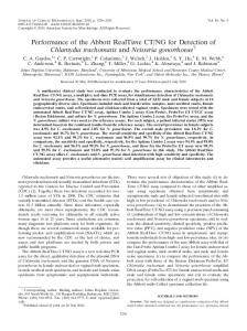
dates. For reference, Figures 2 to 5 plot the values of the real-time recession probabilities used to date each peak and trough in the sample. That is, these figures show a sequence of P( S t = 1 | ΨT ) that was available at the vintage for which the business cycle peak or trough was first identified.
4.4 Revisions of Business Cycle Dates The NBER’s business cycle dating committee has never revised an established business cycle turning point date, despite the fact that economic data is often revised substantially. Does this rigidity suggest that the NBER’s business cycle dates are no longer consistent with the data? We can evaluate the importance of data revisions for business cycle turning point dates by tracking revisions to the dates established using the MHP algorithm and DFMS model. In particular, for each dating method, Tables 5 and 6 give the initial business cycle date established (taken from Tables 3 and 4) and the business cycle date established using the most recent vintage of data available (taken from Tables 1 and 2). To assess the NBER’s practice of not revising turning point dates, we are particularly interested in the impact of data revisions occurring after the NBER’s announcement. Thus, we also list the business cycle date established by each dating method at the vintage closest to the date of the NBER announcement. Note that this is not available in those cases for which the initial date established by the dating method was not available until after the NBER announcement. We begin with Table 5, which contains the results for the MHP algorithm. Comparing columns 2 and 3 with column 4, we can see that there are some fairly large revisions of business cycle dates, with several revisions of 2-3 months and a largest revision of 6 months. However, in most cases these revisions reflect the turning point date established in real time moving closer to
16
the NBER date. Thus, these revisions are not suggestive that the NBER dates themselves require revision. Table 6 contains the results for the DFMS model. In all cases, the dates recorded in real time or at the time of the NBER announcement are within one month of those established using the last vintage of data available, suggesting that revisions of business cycle turning point dates are relatively unimportant. Overall, these results validate the NBER practice of not revising business cycle turning point dates once they are established.
4. Conclusions
This paper investigates the ability of formal rules to establish business cycle turning point dates in real time. Both methods studied, a non-parametric algorithm given in Harding and Pagan (2002) and the dynamic factor Markov-switching model as in Chauvet (1998), accurately identify the NBER turning point dates in real time, with no instances of false positives. Both approaches also provide improvements over the NBER in the timeliness with which they identify business cycle troughs, but provide no such improvement for business cycle peaks. Comparing the two methods, the dynamic factor Markov-switching model identifies NBER turning point dates the most accurately, as well as identifies business cycle troughs with the largest lead.
17
References
Boehm, E. and G.H. Moore, 1984, New Economic Indicators for Australia, 1949-1984, The Australian Economic Review, Fourth Quarter, 34-56. Bry, G. and Boschan, C., 1971, Cyclical Analysis of Time Series: Selected Procedures and Computer Programs, New York: National Bureau of Economic Research. Burns, A.F. and W.A. Mitchell, 1946, Measuring Business Cycles (NBER, New York). Chauvet, M., 1998, An Econometric Characterization of Business Cycle Dynamics with Factor Structure and Regime Switching, International Economic Review 39, 969-996. Chauvet, M., 2001 “A Monthly Indicator of Brazilian GDP,” The Brazilian Review of Econometrics 21 (1), 1-15. (Revista de Econometria). Chauvet, M. and J. Piger, 2003, Identifying Business Cycle Turning Points in Real Time, Federal Reserve Bank of St. Louis Review 85, 47-61. Chauvet, M. and J. Hamilton, 2004, Dating Business Cycles in Real Time, mimeo, University of California, Riverside. Croushore, D. and T. Stark, 2001, A Real-Time Data Set for Macroeconomists, Journal of Econometrics 105, 111-130. Hamilton, J.D., 1989, A New Approach to the Economic Analysis of Nonstationary Time Series and the Business Cycle, Econometrica 57, 357-384. Harding, D. and A. Pagan, 2002, Synchronization of Cycles, mimeo. Harding, D. and A. Pagan, 2003, A Comparison of Two Business Cycle Dating Methods, Journal of Economic Dynamics and Control 27, 1681-1690. Kim, C.-J., 1994, Dynamic Linear Models with Markov-Switching, Journal of Econometrics, 60, 1-22. Kim, C.-J. and C.R. Nelson, 1998, Business Cycle Turning Points, a New Coincident Index, and Tests of Duration Dependence Based on a Dynamic Factor Model with Regime Switching, The Review of Economics and Statistics 80, 188-201. Layton, A. P., 1996, Dating and Predicting Phase Changes in the U.S. Business Cycle, International Journal of Forecasting 12, 417-428. Mariano, R. M. and Y. Murasawa, 2003, A New Coincident Index of Business Cycles Based on Monthly and Quarterly Series, Journal of Applied Econometrics, 18(4), 427-443.
18
Stock, J.H. and M.W. Watson, 1989, “New Indexes of Coincident and Leading Economic Indicators,” NBER Macroeconomics Annual, 4, 351-393. Watson, M.W, 1994, "Business Cycle Durations and Postwar Stabilization of the U.S. Economy," American Economic Review, 84, 24-46.
19
Appendix: Sources of Real-Time Data
Real Personal Income Excluding Transfer Payments For vintages from December 1976 through March 1990, data for real personal income was collected from Business Conditions Digest, while for vintages from April 1990 through December 1995, real personal income data was collected from the Survey of Current Business. For vintages from January 1996 through November 2003, real personal income data was collected from Business Cycle Indicators and data archives maintained by the Federal Reserve Bank of Saint Louis. In some cases for vintages from January 1996 onward, only nominal personal income and real and nominal personal disposable income data were available. To obtain real personal income data, we deflated nominal personal income by real-time data for the ratio of nominal to real personal disposable income, which was collected from the Survey of Current Business. We were only able to obtain real-time data on real transfer payments for a limited number of vintages. To exclude transfer payments we assume that transfer payments data is not revised except for level shifts. This assumption allows us to use the ratio of nominal personal income to transfer payments obtained from the latest vintage in our sample, November 2003, to exclude transfer payments from all earlier vintages. For those vintages for which we were able to collect the actual transfer payments data, we compared this data to the approximations and found them to be quite accurate.
Real Manufacturing and Trade Sales For vintages from December 1976 through March 1990, data for real manufacturing and trade sales was collected from Business Conditions Digest, while for vintages from April 1990
20
through December 1995, real manufacturing and trade sales data was collected from the Survey of Current Business. For vintages from January 1996 through November 2003, real manufacturing and trade sales data was collected from Business Cycle Indicators, Business Statistics, and the Survey of Current Business. For a small number of individual vintages, there were gaps in the data available. This missing data was filled in using the following strategy: Define the missing data for month t at vintage R as Yt R . Suppose that data is available for Yt R − h and Yt R + g , as well as for Yt +Rk− h , Yt +Rk , and Yt +Rk+ g . To obtain an imputed value of Yt R , denoted Yˆt R , we use the following geometric average:
Yˆt R = Yt R − h * r1 * Yt R + g * r2 , where r1 =
Yt +Rk−1 Yt +Rk+1 r and = . 2 Yt +Rk Yt +Rk
21
1.0
0.8
0.6
0.4
0.2
0.0 1970
1975
1980
1985
1990
1995
2000
Figure 1: Full Sample Smoothed Probabilities of Recession and NBER Recessions (Shaded).
22
1.0
0.8
0.6
0.4
0.2
0.0 1979:01
1979:07
1980:01
1980:07
1981:01
Figure 2: Real Time Probabilities of Recession Determining the Peak (___) and Trough (---) of the 1980 Recession, and NBER Recession (Shaded).
1.0
0.8
0.6
0.4
0.2
0.0 81:01
81:07
82:01
82:07
83:01
83:07
Figure 3: Real Time Probabilities of Recession Determining the Peak (___) and Trough (---) of the 1981-82 Recession, and NBER Recession (Shaded).
23
1.0
0.8
0.6
0.4
0.2
0.0 1990:01
1990:07
1991:01
1991:07
1992:01
Figure 4: Real Time Probabilities of Recession Determining the Peak (___) and Trough (---) of the 1990-91 Recession, and NBER Recession (Shaded).
1.0
0.8
0.6
0.4
0.2
0.0 00:01
00:07
01:01
01:07
02:01
02:07
03:01
Figure 5: Real Time Probabilities of Recession Determining the Peak (___) and Trough (---) of the 2001 Recession, and NBER Recession (Shaded).
24
Table 1 Business Cycle Dates: NBER and MHP Algorithm Data sample: January 1967 – September 2003; Data vintage: November 2003
Peaks
Troughs
MHP
NBER
Lead / Lag Discrepancy
MHP
NBER
Lead / Lag Discrepancy
Dec 1969
Dec 1969
0M
Nov 1970
Nov 1970
0M
Nov 1973
Nov 1973
0M
Mar 1975
Mar 1975
0M
Oct 1979
Jan 1980
3M
Jul 1980
Jul 1980
0M
Jul 1981
Jul 1981
0M
Dec 1982
Nov 1982
-1M
Jul 1990
Jul 1990
0M
Jan 1991
Mar 1991
2M
Dec 2000
Mar 2001
3M
Nov 2001
Nov 2001
0M
25
Table 2 Business Cycle Dates: NBER and DFMS Model Data sample: January 1967 – September 2003; Data vintage: November 2003
Peaks
Troughs
DFMS
NBER
Lead / Lag Discrepancy
DFMS
NBER
Lead / Lag Discrepancy
Oct 1969
Dec 1969
2M
Oct 1970
Nov 1970
1M
Dec 1973
Nov 1973
-1M
Mar 1975
Mar 1975
0M
Jan 1980
Jan 1980
0M
Jul 1980
Jul 1980
0M
Jul 1981
Jul 1981
0M
Nov 1982
Nov 1982
0M
Jul 1990
Jul 1990
0M
Mar 1991
Mar 1991
0M
Nov 2000
Mar 2001
4M
Dec 2001
Nov 2001
-1M
26
Table 3 Business Cycle Dates Obtained in Real Time – NBER and MHP Algorithm
Peak Date: MHP Jul 1979
Peak Date: NBER Jan 1980
Lead / Lag Discrepancy
May 1981
6M
Peak Date Available: MHP Jun 30, 1980
Peak Date Announced: NBER Jun 3, 1980
Days ahead of NBER Announcement -27
Jul 1981
2M
Mar 31, 1982
Jan 6, 1982
-84
Jul 1990
Jul 1990
0M
Apr 30, 1991
Apr 25, 1991
-5
Sep 2000
Mar 2001
6M
Dec 31, 2001
Nov 26, 2001
-35
Trough Date: MHP Jul 1980
Trough Date: NBER Jul 1980
Lead / Lag Discrepancy 0
Trough Date Available: MHP May 31, 1981
Trough Date Announced: NBER Jul 8, 1981
Days ahead of NBER Announcement 38
Oct 1982
Nov 1982
1M
Aug 31, 1983
Jul 8, 1983
-54
Jul 1991
Mar 1991
-4M
Mar 31, 1992
Dec 22, 1992
266
Nov 2001
Nov 2001
0M
Sep 30, 2002
July 17, 2003
290
27
Table 4 Business Cycle Dates Obtained in Real Time – NBER and DFMS Model
Peak Date: DFMS Jan 1980
Peak Date: NBER Jan 1980
Lead / Lag Discrepancy
Aug 1981
0M
Peak Date Available: DFMS Jul 31, 1980
Peak Date Announced: NBER Jun 3, 1980
Days ahead of NBER Announcement -58
Jul 1981
-1M
Feb 28, 1982
Jan 6, 1982
-53
Aug 1990
Jul 1990
-1M
Mar 31, 1991
Apr 25, 1991
25
Nov 2000
Mar 2001
4M
Jan 31, 2002
Nov 26, 2001
-66
Trough Date: DFMS Jun 1980
Trough Date: NBER Jul 1980
Lead / Lag Discrepancy 1M
Trough Date Available: DFMS Dec 31, 1980
Trough Date Announced: NBER Jul 8, 1981
Days ahead of NBER Announcement 189
Nov 1982
Nov 1982
0M
May 31, 1983
Jul 8, 1983
38
Mar 1991
Mar 1991
0M
Sep 30, 1991
Dec 22, 1992
448
Nov 2001
Nov 2001
0M
Aug 31, 2002
July 17, 2003
320
28
Table 5 Revisions to Business Cycle Dates: MHP Algorithm Initial Date: MHP
Date at Vintage Closest to NBER Announcement: MHP
Date at Final Vintage: MHP
Jan 1980
Jul 1979
NA
Oct 1979
Jul 1981
May 1981
NA
Jul 1981
Jul 1990
Jul 1990
NA
Jul 1990
Mar 2001
Sep 2000
NA
Dec 2000
Jul 1980
Jul 1980
Jul 1980
Jul 1980
Nov 1982
Oct 1982
NA
Dec 1982
Mar 1991
Jul 1991
Feb 1991
Jan 1991
Nov 2001
Nov 2001
Nov 2001
Nov 2001
NBER Date Peaks
Troughs
29
Table 6 Revisions to Business Cycle Dates: DFMS Model Initial Date: DFMS
Date at Time of NBER Announcement: DFMS
Final Date: DFMS
Jan 1980
Jan 1980
NA
Jan 1980
Jul 1981
Aug 1981
NA
Jul 1981
Jul 1990
Aug 1990
Aug 1990
Jul 1990
Mar 2001
Nov 2000
NA
Nov 2000
Jul 1980
Jun 1980
Jun 1980
Jul 1980
Nov 1982
Nov 1982
Nov 1982
Nov 1982
Mar 1991
Mar 1991
Mar 1991
Mar 1991
Nov 2001
Nov 2001
Jan 2002
Dec 2001
NBER Date Peaks
Troughs
30