In this paper, we propose an adaptive scheduling framework, compensation-based scheduling, to provide predictable execution times by using feedback control.
A Compensation-based Scheduling Scheme for Grid Computing Y.M. Teo1,2, X. Wang1,2 and J.P. Gozali1 1
2
Department of Computer Science, National University of Singapore, Singapore 117543 Singapore-Massachusetts Institute of Technology Alliance, 4 Engineering Drive 3, Singapore 117576 {teoym, wangxb}@comp.nus.edu.sg
Abstract Wide fluctuations in the availability of idle processor cycles and communication latencies over multiple resource administrative domains present a challenge to provide quality of service in executing grid applications. In this paper, we propose an adaptive scheduling framework, compensation-based scheduling, to provide predictable execution times by using feedback control. The compensation-based scheduling compensates resource loss during application execution by dynamically allocating additional resources. The framework is evaluated by experiments conducted on the ALiCE scheduler. Scalability simulation studies show that the gaps between actual and estimated execution times are reduced to less than 15% of the estimated execution times.
1
Introduction
Providing predictable execution times is a challenge in grids due to wide fluctuations in resource capacities [22]. Network bandwidth and latencies may change depending on traffic patterns of the Internet. The availability of idle CPU cycles also varies depending on local resource usage. With such fluctuations, there is no certainty when a grid task or job will complete its execution. Application execution times, therefore, become unpredictable. There are three main scheduling approaches for achieving predictable execution times in grids. Advanced reservation [9], used in Silver [21] and Interleaved Hybrid Scheduling [10], aims to build mechanisms for requesting exclusive use of a portion of the capacity of a resource for grid jobs, and therefore avoid having fluctuating shared resource capacities. The drawback of this approach is that not all local schedulers provide advanced reservation support. The second is predictive techniques implemented in the Network Weather Service [14], [29]. It uses statistical extrapolation of historical measurement data to forecast processor utilization and network bandwidth. Grid schedulers use this information to estimate application
execution time and perform scheduling [18], [19]. AppLeS [20] and EveryWare [28] are examples of predictive technique-based systems. The predictive approach assumes that performance data of past executions of applications on known resources are available. This assumption, however, is not practical since there are scenarios where resources join and leave the grid at any time, or where there are new applications submitted for execution. This technique is also difficult to implement since most current systems do not provide the additional information required by predictive techniques [17]. The third is feedback control, which is an approach widely used in engineering to obtain high performance in the presence of uncertainty. The key idea is to compare measured performance with the desired performance and to perform corrections dynamically. CHAIMS [12], a service-centered grid, represents local resources as service providers and grid tasks are represented as service requests, is one system that uses feedback control. It monitors service fulfillment progress and uses the information to repair schedules. GrADSoft [2], [6] is another system that uses the feedback control approach. It provides an application development environment for building grid jobs that can automatically adapt to changing grid environments. The feedback control approach has several advantages over advanced reservation and predictive techniques. First, it requires no additional support from local schedulers. Hence, a grid scheduler implementing this approach can interface with any local scheduler. Second, it does not require data of past application executions. Therefore, a grid scheduler can provide predictable execution times for grid applications that have not been previously executed. Despite the advantages of the feedback control scheduling approach, such systems require extensive use of application development and profiling tools. Both CHAIMS and GrADSoft use complex methods for application performance monitoring and schedule corrections. This results in complex frameworks for application development. These frameworks include special compilers and application toolkits that might be
Y.M. Teo, X. Wang and J.P. Gozali, A Compensation-based Scheduling Scheme for Grid Computing, Proceedings of the 7th International Conference on High Performance Computing and Grid, pp. 334-342, IEEE Computer Society Press, Tokyo, Japan, July 20-22, 2004.
1
difficult for new application developers to learn and use. Therefore, there is a need for simpler methods based on commodity technologies that do not introduce new application development frameworks. In this paper, we propose a feedback control adaptive scheduling framework, compensation-based scheduling, using a simple yet novel compensation method for schedule corrections. The framework is implemented in ALiCE [[1], [25]], our Java-based commodity grid middleware, as the ALiCE scheduler. We also implemented an ALiCE simulator, which uses the process-oriented simulation paradigm in modeling the compensation-based scheduler and the grid environment. The results and analysis of our experiments show that the compensation-based framework is able to provide predictable execution times despite the existence of wide resource capacity fluctuations. We also investigate the effects of various resource and application parameters on scheduler performance. The rest paper is organized as follows. Section 2 describes the proposed compensation-based scheduling. Section 3 presents the implementation of the framework in ALiCE, the ALiCE scheduler and the ALiCE simulator. Section 4 presents the experimental analysis. Our concluding remarks are in section 5.
2
Compensation-based Scheduling
2.1 Framework Overview The compensation-based scheduling framework, illustrated in Figure 1, extends the two-level scheduling architecture discussed by Feitelson in [7] into three levels. Grid Information Service
Resource Information Table
Grid User
applications
Deadline Estimator
deadline
Local Scheduler
Resource Compensator
| | | |
application performance
Meta-scheduler
| | | | resource allocation
Performance Monitor
Administrative domain
Local Scheduler
| | | |
Jobs/tasks
Shared Resource
Shared Resource
Administrative domain
Application Scheduler Job/Task Pool Jobs/tasks
| | | |
Local Scheduler
| | | |
Shared Resource
applications, and ensuring that the resource requirement of each application is met. The second level consists of an application scheduler that schedules tasks by interfacing with the local schedulers of the grid resources. The application scheduler maps tasks to shared resources. The third level of scheduler consists of the autonomous local-schedulers that schedule both local and grid tasks on shared resources. The decoupling of an application scheduler and the meta-scheduler is a fundamental concept behind compensation-based scheduling. With this approach, we can use scheduling policies widely available in the literature for parallel job allocations [8] in the application scheduler. The framework includes another three key components: • Execution time Estimator (Deadline Estimator): Provides application execution time estimates. • Performance Monitor: Application performance is monitored such that capacity fluctuations can be compensated. • Resource Compensator: In response to changes in monitored application performance, modifications to resource allocations are made. Two external factors that serve as inputs to the framework are applications and shared resources. The framework is applicable to master-slave type of applications represented by two parameters: number of tasks and task sizes. A task is an entity of work that is to be executed by the system. Task dependencies are not considered as an application parameter in the framework. Predicting execution time with task dependencies is discussed in [18]. Task size is the amount of work that has to be done by the processors of shared resources to execute the task. Shared resources are represented in the framework by the two parameters: computational capacity, and communication delay. Computational capacity defines the computational power of a resource based on the Linpack benchmark [13]; it is measured in Millions of Floatingpoint Operations per Second (MFLOPS). Communication delay is the amount of time required for a grid scheduler to deliver a message of minimum size to the resource; it is measured in milliseconds. The Grid Information Service [4] is a repository for information about grid resources. It normally consists of two main components: a set of sensors to capture resource information, and a directory service to allow efficient retrieval of resource information.
Administrative domain
Grid Scheduler
Grid Resources
Figure 1. Compensation-based Scheduling Framework The first level consists of a meta-scheduler that oversees the scheduling of multiple applications, the partitioning of available resources among these
2.2 Execution Time Estimator The execution time estimator provides an estimate of the time required to complete the execution of an application. A key challenge is to provide an accurate estimate in spite of fluctuating resource capacities, and not knowing the task sizes.
Y.M. Teo, X. Wang and J.P. Gozali, A Compensation-based Scheduling Scheme for Grid Computing, Proceedings of the 7th International Conference on High Performance Computing and Grid, pp. 334-342, IEEE Computer Society Press, Tokyo, Japan, July 20-22, 2004.
2
Our algorithm first obtains available resources from the meta-scheduler. The set of available resources is then used to execute N randomly selected tasks, where N is the size of the available resource set given by the metascheduler. We then execute these N tasks on the set of available resources using the meta-scheduling policy. The measured execution times are used as a first approximation of the execution time of the entire application.
2.3 Meta and Application Schedulers In our proposed framework, scheduling is divided into two steps: resource allocation, handled by the metascheduler, and task assignment, handled by the application scheduler. Resource allocation is the process of allocating resources to an application. Resources allocated to an application are divided into two sets: an execution pool, and a compensation pool. Task assignment is the process of assigning the tasks of an application to resources in the execution pool of the application. Prior to allocating resources to applications, the metascheduler divides shared grid resources into several partitions of equal size. During resource allocation, two partitions are assigned as the execution and compensation pools respectively. An execution pool of an application belongs exclusively to that application. The exclusive usage of execution pools enables us to influence the performance of an application by adding or removing resources from its execution pool. A compensation pool, however, may be shared by many applications. The maximum number of applications sharing a compensation pool is called the Degree of Overlap (DOO). The most conservative configuration is when DOO = 1. Because partitions are nearly equal in size, this scenario attempts to provide a backup for every resource in the execution pool of an application. Larger values of DOO imply greater sharing of resources in compensation pools. The sharing of compensation pools increases the possible utilization of resources. However, it reduces the effective amount of resources available for compensation of each application. The reduction makes applications more vulnerable to resource capacity fluctuation. The meta-scheduler divides shared grid resources into DOO+1 partitions. This allows a maximum of DOO number of applications to run concurrently and use 1 partition for compensation. Partitions are created dynamically by inserted new producers (compute resources) into the partition with the lowest aggregate capacity. This method creates partitions of near equal capacities. The meta-scheduler assigns partitions to a new application based on these rules:
• If two free partitions are available, assign one as execution pool and the other as compensation pool; • If only one free partition is available, assign the partition as execution pool. Let the new application share the compensation pool of another application. Distribute the sharing of compensation pools equally among currently allocated compensation pools; • If no partitions are available, reject the application. One feature of our framework is that resource allocation (i.e. compensation and deallocation) only changes the configuration of a job’s resource pool. It is worth noting that a job is a set of tasks, and though resource allocation affects a job, it does not affect the running tasks of that job. Running tasks are never migrated during compensation, they are executed until completion. Only previously unallocated tasks get to run on newly added resources. Running tasks are also never cancelled during deallocation because only idle resources are deallocated.
2.4 Performance Monitor The performance monitor measures the execution progress of an application. It calculates the execution rate of an application periodically. The application execution rate of an application A at the nth period, ApprateA(n), is given by the following formulas. if (n − nlast) · tinterval ≤ avg_comp and Rn > 0 Rn α ⋅ Apprate A ( nlast ) Apprate A ( n) = + C ( n) ⋅ t int erval ⋅ (n − nlast ) C ( n) else if (n − nlast) · tinterval ≤ avg_comp and Rn = 0, ApprateA(n) = ApprateA(nlast) otherwise Apprate A (nlast ) ⋅ C ( nlast ) Apprate A (n) = C (nlast ) + (n − nlast ) Rn is the number of tasks that have completed execution since the execution rate is last calculated. tinterval is the length of time between successive calculations of the execution rate. α is the sensitivity factor that ranges from 0 to 1. avg_comp is the average task execution time. nlast is the most recent interval in which a task completed its execution. C(n) is (1 − αn) ⁄ (1 − α) the sum of the geometric series between 1 to n with α as the ratio, and ApprateA(0) is set to zero. The application execution rate computation is designed to achieve two purposes: responsive to sudden changes in resource capacity information derived from task completion events, and to gradually decrease in the absence of task completion events. The first purpose is addressed in the first equation where past task completion events are given the weight of α. The choice of α value determines the ratio between the
Y.M. Teo, X. Wang and J.P. Gozali, A Compensation-based Scheduling Scheme for Grid Computing, Proceedings of the 7th International Conference on High Performance Computing and Grid, pp. 334-342, IEEE Computer Society Press, Tokyo, Japan, July 20-22, 2004.
3
use of previous application execution rate calculations and the new information required since nlast, the most recent interval that a task completes execution. The smaller the value of α, the more sensitive the calculation is to recent events. The second purpose is such that the application execution rate value captures delayed task completion events caused by reduction in shared resource capacity. Delayed task completion events are assumed when no task completion events occur after avg_comp time has passed since nlast, that is when (n − nlast) · tinterval > avg_comp. During avg_comp time since nlast, the application execution rate does not decrease as shown in the second formula. After this has passed, however, the application execution rate calculation uses the third formula, which results in the execution rate to gradually decrease over time. This decrease continues until a task completes execution, which resets the nlast value and thus forces the calculation of the execution rate to use the first formula.
2.5 Resource Compensator The resource compensator performs resource reallocation in response to changes in monitored application performance. Reallocation of resources falls into two categories: compensation and deallocation. Compensation occurs when actual application performance results in an execution time that is greater than the estimated execution time. In this case, additional resources are allocated to compensate the performance loss. The issues involved in this process are in distinguishing transient from permanent performance loss, and determining which spare resources to allocate. Deallocation occurs when application performance results in execution time that is less than what is estimated. In this case, the scheduler must deallocate resources so that applications that are lacking resources can benefit. The main issue is in detecting applications with excess resource and determining which resources to deallocate. The various methods for implementing the resource compensator are differentiated by: how they check the application performance, how they prioritize applications, and the preconditions that must be satisfied before resource allocation or deallocation can take place. The method we choose periodically checks application performance at a static interval determined by the grid system administrator. The choice of interval length affects system performance as well as the accuracy of the monitoring. The shorter the interval, the more sensitive the resource compensator will be to changes in application execution rate, and at the same time the more CPU time it utilizes. We prioritize applications with the earliest execution time estimate, i.e. the shorter the distance between the
estimated execution time of an application and current time, the higher priority the application has. We allocate resources in response to reduction in application performance immediately, but we only deallocate resources from applications whose estimated execution times are still far from the current time. At every interval, the algorithm runs through a list of running applications in order of their estimated execution times; the application with the nearest estimated execution time is checked first and the application with the longest estimated execution time is checked last. For each of these applications, the resource compensator uses the performance monitor to obtain application performance and calculates the estimated time for application completion. If the estimated execution time is later than the sum of the application start time and estimated execution time, then the resource compensator allocates a new resource to the application. By going through the application list in order of nearest estimated completion time, the resource compensator gives critical applications higher priorities. The reasoning behind this is that applications with nearer estimated completion times have fewer chances for compensations whereas applications with estimated completion times that are further away still have more chances for compensations. The algorithm also checks for overcompensation – the over-allocation of resources that will make the application be completed much sooner than the user-chosen completion time. It handles this situation by checking for conditions where the application execution rate is greater than or equal to one and a half times of what is required to complete the execution within the user-chosen estimated completion time. When this occurs, the resource with the minimum capacity is removed from the execution pool of the application. The resource with the minimum capacity is chosen to avoid deallocating too many resources. Since deallocating too many resources may cause the application to complete execution later than the userchosen estimated completion time, the algorithm avoids deallocation of resources altogether at the final stages of the application execution.
2.6 Performance Metrics The performance of a compensation-based scheduler is measured using three metrics: • Estimated Execution Time Miss Ratio (EETMR), the ratio between the number of applications that has missed their estimated completion times and the total number of applications executed; an application is considered to have missed its estimated completion time if it completes execution later by 1% or more of the estimate.
Y.M. Teo, X. Wang and J.P. Gozali, A Compensation-based Scheduling Scheme for Grid Computing, Proceedings of the 7th International Conference on High Performance Computing and Grid, pp. 334-342, IEEE Computer Society Press, Tokyo, Japan, July 20-22, 2004.
4
• Average Completion Gap (ACG), the average absolute time difference between actual and estimated execution times divided by the estimated application execution time; • Total Execution time (TET), the sum of execution times of all applications submitted to the scheduler. EETMR captures the ability of the scheduler to complete job executions by their estimated completion times. Its values range from zero to one, and are obtained by dividing the number of execution time estimation misses by the number of applications submitted. Low EETMR values imply fewer execution time estimation misses occurred; thus, the scheduler has high ability of completing job executions by the estimated completion times. ACG captures the predictability of application execution times. Its values range from zero to one, and are obtained by the formula: 1 n | est _ execi − execi | ACG = ∑ n i =1 est _ execi where n is the number of applications in the experiment; execi and est_execi are the actual and estimated execution time application i respectively measured in seconds. The closer ACG is to zero, the more predictable application execution times are. Total Execution time (TET) is obtained from the formula: n
TET = ∑ execi i =1
where n is the number of applications in the experiment; execi is the execution time of application i respectively measured in seconds. TET captures the system throughput; lower values indicate higher throughput.
3
Scheduler Implementation in ALiCE
ALiCE (Adaptive and scaLable internet-based Compute Engine) [[1], [25]] is our Java-based commodity grid middleware. It uses Java, Jini [27], and JavaSpaces [24] to provide core-grid and user-level middleware services. ALiCE consists of two main components: a platform independent runtime system that manages computational grid resources and a set of programming templates for development of parallel Java grid applications. In this section, we discuss two implementations of the framework: in the ALiCE grid system and in the grid simulator we have developed.
and resource information, the scheduler queries information providers such as the Producer Manager and Task Manager. Figure 2 shows the compensation-based ALiCE scheduler architecture and interfaces with other broker components. Producer Manager
Information Query Interface
Execution Time Estimator
Application Submission Interface
Application Manager
Execution Monitoring Interface
Performance Monitor
Job/Task Executor
Resource Compensator Application Schedulers
Meta-scheduler
Schedule Execution Interface
Grid Scheduler
Figure 2. Compensation-based ALiCE Scheduler Four main interfaces are application submission, execution monitoring, schedule execution, and information query. The application submission interface links the Application Manager, the ALiCE component that handles application submission, with the execution time estimator and meta-scheduler. The Application Manager uses the interface to query estimated application execution time from the execution time estimator. The estimated application execution time is then returned to the user. If the user accepts the estimate, the Application Manager will send the application to the meta-scheduler. The execution monitoring interface is used by the performance monitor to obtain application execution progress from the Job/Task Executor. The schedule execution interface is used by application scheduler to invoke the job/task executors to start execution of jobs or tasks. The information query interface is used for scheduler components to enquire about producer and task information. Figure 3 shows the conceptual class diagram for scheduler components and their main methods. ApplicationManager 1
1 0 ..*
1
1 ExecutionTimeEstimator +estimate()
ResourceCompensator
PerformanceMonitor
+register() +deregister()
+getApplicationRate() 1 Executor
1
+executeTask()
3.1 ALiCE Scheduler Our goal is to implement the ALiCE scheduler using the compensation-based scheduling framework. The scheduler is part of the resource broker; therefore, it has to collaborate with resource broker components to achieve its function. For example, to obtain application
Other Information Providers
Task Manager
1
MetaScheduler 1
1 +createPartition() +getNextAllocation() +registerApplication() +cleanupExecution()
1
1
ApplicationScheduler 0 ..* +addProducer(): +removeProducer() +addTask()
0 ..*
Figure 3. Scheduler Class Diagram
Y.M. Teo, X. Wang and J.P. Gozali, A Compensation-based Scheduling Scheme for Grid Computing, Proceedings of the 7th International Conference on High Performance Computing and Grid, pp. 334-342, IEEE Computer Society Press, Tokyo, Japan, July 20-22, 2004.
5
Four scheduling policies are implemented in the ALiCE scheduler: eager scheduling [3], trapezoidal self scheduling [26], guided self scheduling [16], and factoring [11].
3.2 simALiCE: the ALiCE Grid Simulator simALiCE is a simulator of the ALiCE Grid System. It simulates a compensation-based scheduler. simALiCE is developed using the SPaDES/Java [23] library, an implementation of the SPaDES (Structured Parallel Discrete-event Simulation) modeling and simulation framework based on the process-oriented modeling paradigm. simALiCE models the ALiCE computational grid. This simALiCE grid simulation model consists of applications, producers (or compute nodes), and the scheduler as shown in Figure 4. An application is modeled by its arrival time, number of tasks, and task size. Task size is used to calculate execution time. Producers are represented by seven parameters illustrated in Table 1.
Figure 5 shows the simALiCE architecture with three main components: simulation kernel, simulation processes, and the output statistics collector. The simulation kernel is responsible for reading the simulation configuration file, initializing the simulation processes, starting the simulation, stopping the simulation after the simulation duration has passed, and monitoring the output statistics for the simulation. Simulation processes models the ALiCE grid system entities that we simulate. The output statistics collector contains mechanisms for collecting the three output statistics we mentioned earlier: EETMR, TET, and ACG.
Resource Compensator Process
Simulation Kernel
Producer
Application Application Application Process Process Processes
Scheduler Process
Task Task Task Process Process Processes
Task Task ProducerLink Process Process Processes
Task Task Producer Process Process Processes
Output Statistics Collector
Simulation Processes
tasks
Figure 5: simALiCE Architecture tasks Producer
tasks Scheduler
Producer
Applications
Figure 4. simALiCE Grid Simulation Model Parameter COMP_CAPbench COMP_CAPeff FLUC_SIZEcomp FLUC_INTcomp COMM_DELAY
FLUC_SIZEcomm. FLUC_INTcomm.
Description Values Benchmarked Computational MFLOPS Capacity Effective Computational Capacity work unit per ms Maximum Computational Capacity Percentage Reduction Computational Capacity Fluctuation Millisecond Interval Benchmarked Communications Millisecond Delay between Scheduler and Producer Max Communications Delay Increase Percentage Communications Delay Fluctuation Millisecond Interval
Table 1. Compute Node Parameters The communication refers to the link between the producer and the scheduler. The scheduler parameters are the degree of overlap, monitoring interval length, whether compensation is enabled, and the scheduling policy used. Four policies modeled in simALiCE are: eager scheduling (ES), trapezoidal self scheduling (TSS), guided self scheduling (GSS), and factoring (FAC2).
The application process models the activity of a running application. This process is created by the simulation kernel based on the application parameters specified in the configuration file. The task process models the activity of a task. It is created by the application process. Producer processes model the activity of ALiCE producers. Producer link processes model the communication link between an ALiCE producer and the scheduler. Where the producer processes maintain computational capacity values, producer link processes maintain communication delay values. The scheduler process implements the meta-scheduler and application scheduler components of the compensation-based scheduling framework. The resource compensator process models the resource compensator and performance monitor components of the compensationbased scheduling framework. The simulator has been verified and has shown no inconsistencies with real-life ALiCE runs. Slight inaccuracies in numerical results, however, may arise due to the lack of precision in our measurements.
4
Experimental Analysis
The main aim of the experiments is to show the effectiveness of compensation-based under wide resource capacity fluctuations. To achieve our objective, we carried out one set of experiments on the real ALiCE
Y.M. Teo, X. Wang and J.P. Gozali, A Compensation-based Scheduling Scheme for Grid Computing, Proceedings of the 7th International Conference on High Performance Computing and Grid, pp. 334-342, IEEE Computer Society Press, Tokyo, Japan, July 20-22, 2004.
6
system and scalability experiments are performed on the simALiCE simulator. In this experiment, we use DESKey, a grid program in Java that searches for a DES [15] encryption key by brute-force checking of every key in a defined key-space [5]. DESKey has two main parameters: LENGTH and NUMKEYS. The first refers to the length of the DES key in bits; it determines the size of the key-space to be searched, and therefore, determines the total execution time of the application. For a key length of n, the number of keys to be checked is 2n. NUMKEYS is the number of keys per task. In this section, we investigate the DESKey program with LENGTH = 28-bit and NUMKEYS = 10 millions.
4.1 Experiments on ALiCE scheduler The experiment uses a cluster of sixteen nodes: eight Intel Pentium III, 866 MHz (COMP_CAPbench = 85 MFLOPS) and eight Pentium 4 2.4 GHz (COMP_CAPbench = 137 MFLOPS) nodes. Two of the Pentium 4 nodes are used to host the resource broker components while other nodes are used as producers. To emulate computational resource capacity fluctuations, an artificial load-generator is used. The load-generator has two parameters: MAXJOB and FLUC_INT. MAXJOB defines the maximum number of background jobs the load-generator has on a cluster node. The number of jobs is modeled using a uniform distribution. Each background
Experiment
Two jobs
Three jobs
Eight jobs
Load Generator Parameters FLUC_INT MAXJOB (sec) 0 N.A. 30 1 60 150 30 3 60 150 0 N.A. 30 1 60 150 30 3 60 150 0 N.A. 30 1 60 150 30 3 60 150
job performs compute intensive calculations that takes up CPU time. FLUC_INT defines the length of interval between changes in the number of background jobs. All user jobs running on the cluster are set with equal process priority. Therefore, with MAXJOB = N, the minimal capacity available for a grid job is 100/(N+1)%. For example, when MAXJOB = 3, the minimum capacity available is 25%. The amount of CPU capacity available to grid applications, therefore, can be reduced by increasing N. Due to the limitations of the amount of resources available, only a maximum of eight jobs can be run concurrently. For larger number of applications, the experiments are conducted using simulation. The three experiments conducted on the ALiCE scheduler use the eager task scheduling policy with monitoring interval of 30 seconds: • two jobs run concurrently with the eight Intel Pentium III and DOO = 3; • three jobs run concurrently with the eight Intel Pentium III and DOO = 3; • eight jobs run concurrently with the eight Intel Pentium III and six Intel Pentium 4 and DOO = 10. The experiments results are shown in Table 2. The experiment results show compensation-based scheduling effectively reduces application execution time estimation misses, completion gaps, and execution times under wide resource capacity fluctuations. In the ALiCE grid
Without Compensation TET EETMR ACG (sec) 1.0 0.12 2,335 1.0 0.41 3,171 1.0 0.34 2,909 1.0 0.21 2,537 1.0 0.32 4,098 1.0 0.42 4,045 1.0 0.42 3,014 0.66 0.14 3,674 1.0 0.41 5,002 1.0 0.35 4,605 1.0 0.19 3,953 1.0 0.26 5,896 1.0 0.56 5,511 1.0 0.37 5,287 0 0.07 7,437 0.75 0.19 9,906 0.75 0.17 8,862 0.50 0.16 7,680 0.88 0.34 17,867 0.63 0.33 14,675 0.63 0.33 11,364
With Compensation EETMR
ACG
0 0.5 0.5 0.5 1.0 0.5 0.5 0 0.66 0.33 0.33 0.66 0.33 0.33 0 0.38 0.25 0.20 0.75 0.50 0.50
0.08 0.14 0.13 0.12 0.13 0.15 0.12 0.16 0.09 0.12 0.11 0.25 0.31 0.10 0.03 0.24 0.23 0.17 0.38 0.38 0.16
TET (sec) 2,067 2,302 2,187 2,240 3,645 3,314 2,921 3,723 2,163 1,859 1,803 3,556 2,345 2,070 7,309 9,021 8,764 7,243 13,304 11,954 8,461
Table 2. Experiment Results on the ALiCE Grid System Y.M. Teo, X. Wang and J.P. Gozali, A Compensation-based Scheduling Scheme for Grid Computing, Proceedings of the 7th International Conference on High Performance Computing and Grid, pp. 334-342, IEEE Computer Society Press, Tokyo, Japan, July 20-22, 2004.
7
experiments for two jobs on homogeneous resources, execution time estimation misses are reduced by 50% in most cases, total execution times are improved by an average of 21% for MAXJOB = 1 and 11% for MAXJOB = 3, and gap between actual and estimated execution times are narrowed to less than 15% of the estimates. In the ALiCE grid experiment for eight jobs on heterogeneous resources, it is observed that the lack of resources for compensation reduces scheduling performance. Nevertheless, for computational capacity fluctuation size MAXJOB = 3, the ACG is successfully reduced to an average of 0.21. From Table 2, we can make three observations: First, runs with larger fluctuation size, shown with larger MAXJOB, have larger TETs. Second, the ACG values has been successfully reduced to less than 0.20 for most cases except for the case where resources available for compensation is reduced and capacity fluctuation is high with maximum capacity reduction of 75%. Third, we observe the need to improve the execution time estimation algorithm since inaccurate execution time estimations happen even when no resource fluctuations exist. One possible improvement is to incorporate estimation errors into execution time estimates.
applications and 160 producers and DOO = 19 (see Table 4). With more producers and applications, we have a better representation of the performance of compensationbased scheduling. Results for all scenarios in Table 3 show that compensation-based has scheduling narrowed down ACG to less than 0.20; EETMR is reduced to an average of 0.20 for all scenarios. From Table 4, we gain insight on the relationship between size of computational capacity fluctuation, FLUC_SIZEcomp, and improvement in EETMR. The simulation shows that EETMR improvement increases as FLUC_SIZEcomp increases. This is attributed to greater fluctuation resulting in more execution time estimation misses and thus, making more opportunities for compensation-based scheduling to perform compensation. However, when FLUC_SIZEcomp reaches a certain value, the improvement gained from compensation-based scheduling decreases. This decrease is attributed to the lack of resources allocated to the meta-scheduler for compensation. FLUC_SIZE FLUC_INT comp (%) comp (min)
4.2 Scalability Simulation Experiments In our simulation experiment, we model scenarios where an application has a sequential execution time of 2 days. Assuming this job is partitioned into 96 parallel tasks with an average execution time of 30 minutes per task. On eight compute nodes, the parallel execution time is six hours assuming perfect speedup. We present two experiments. The common parameters include COMP_CAPbench = 40, COMP_CAPeff = 10, COMM_DELAY = 1,500, FLUC_SIZEcomm. = 0, FLUC_INTcomm.. = 0, eager task scheduling and the monitoring interval is 4 minutes.
10
Without With Compensation Compensation FLUC_SIZE #Prod #Apps comp(%) EET TET EET TET ACG ACG MR (min) MR (min) 50 0.80 0.26 4,485 0.20 0.11 3,712 160 10 75 1.00 0.49 4,361 0.20 0.16 4,360 50 0.75 0.27 10,043 0.10 0.10 8,014 320 20 75 0.80 0.42 12,077 0.10 0.09 8,850 50 0.75 0.29 17,953 0.20 0.13 14,772 640 40 75 0.85 0.48 21,862 0.25 0.15 17,584
75
Table 3. Varying the Number of Producers and the Number of Applications In the first experiment (see Table 3), we increase the number of producers and applications with FLUC_INTcomp = 5 minutes. In the second experiment, we vary the computational fluctuation parameters with 10
30
50
60
5 15 60 5 15 60 5 15 60 5 15 60 5 15 60
Without Compensation EET TET ACG MR (min) 0.30 0.08 3,534 0.30 0.08 3532 0.20 0.08 3,548 0.80 0.17 3,962 0.70 0.17 3,993 0.80 0.17 3,929 1.00 0.30 4,509 0.90 0.28 4,449 0.80 0.27 4,339 0.90 0.39 4,905 0.80 0.36 4,811 1.00 0.40 4,975 1.00 0.41 5,423 0.90 0.51 5,727 0.90 0.47 5,503
With Compensation EET TET ACG MR (min) 0.20 0.15 3,184 0.20 0.14 3,116 0.20 0.09 3,283 0.20 0.15 3,402 0.20 0.13 3,419 0.20 0.19 2,973 0.30 0.12 3,800 0.20 0.13 3,696 0.10 0.17 3,352 0.20 0.08 3,918 0.30 0.14 3,084 0.20 0.16 3,781 0.30 0.12 4,244 0.40 0.14 4,357 0.30 0.17 4,053
Table 4. Varying Computational Fluctuation Parameters
5
Conclusion
This paper proposes a framework for adaptive grid scheduling with feedback control. The compensationbased scheduling approach provides predictable execution times by monitoring grid application performance, compare the monitored application performance with the desired application performance, and perform corrections by dynamically allocating additional resources. The framework is implemented and evaluated using our ALiCE grid system and scalability is studied using simulation. Experiment results show that compensation-
Y.M. Teo, X. Wang and J.P. Gozali, A Compensation-based Scheduling Scheme for Grid Computing, Proceedings of the 7th International Conference on High Performance Computing and Grid, pp. 334-342, IEEE Computer Society Press, Tokyo, Japan, July 20-22, 2004.
8
based scheduling is effective in reducing execution time estimation misses and total execution times of grid applications. Future works include multi-resource compensation, resource partitioning and allocation, the improvement in the execution time estimator, and the use of heuristics/dynamic methods to determining the value of sensitivity factor in the application execution rate formula.
[17]
References
[19]
[1] ALiCE Grid Computing Project, http://www.comp.nus.edu.sg/~teoym/alice.htm. [2] Berman, F., et al., "The GrADS Project: Software Support for High-Level Grid Application Development", International Journal of High Performance Computing Applications, Volume 15, Number 4, pp. 327-344, 2001. [3] Baratloo, Karaul, Kedem, and Wyckoff, "Charlotte: Metacomputing on the Web", Proceedings of the 9th Conference on Parallel and Distributed Computing Systems, 1996. [4] Czajkowski, K., Fitzgerald, S., Foster, I., Kesselman, C., "Grid Information Services for Distributed Resource Sharing", Proceedings of the Tenth IEEE International Symposium on High-Performance Distributed Computing (HPDC-10), IEEE Press, August 2001. [5] Curtin, M., and Jolske, J., "A Brute Force Search of DES Keyspace", ;login: -- the Newsletter of the USENIX Association, May 1998. [6] Dail, H., Casanova, H., and Berman, F., "A Decoupled Scheduling Approach for the GrADS Program Development Environment", SC2002, 2002. [7] Feitelson, D., "Job Scheduling in Multiprogrammed Parallel Systems", IBM Research Report RC 19970, Second Revision, 1997. [8] Feitelson, D.G., Rudolph, L, Scheiwgelshohn, and Sevcik, K.C., "Theory and Practice in Parallel Job Scheduling", Lecture Notes in Computer Science, 1291, 1997. [9] Foster, I., Roy, A., and Sander, A., "A Quality of Service Architecture that Combines Resource Reservation and Application Adaptation", 8th International Workshop on Quality of Service, 2000. [10] Gehring, J. and Preiss, Th., "Scheduling a metacomputer with un-cooperative subschedulers", In Proc. of IPPS 99 Workshop on Job Scheduling Strategies for Parallel Processing, Lecture Notes in Computer Science, 1999. [11] Hummel, S. F., Schonberg, E., and Flynn, L. E., "Factoring: A method for Scheduling Parallel loops", Communications of the ACM, vol. 35, no. 8, 1992. [12] Keyani, P., Sample, N., and Wiederhold, G., "Scheduling Under Uncertainty: Planning for the Ubiquitous Grid", Technical Report, Stanford Database Group, 2002. [13] Linpack Java, http://www.netlib.org/benchmark/linpackjava/ [14] Lowekamp, B., Miller, N., Sutherland, D., Gross, T., Steenkiste, P., and Subhlok, J., "A Resource Query Interface for Network aware applications", Cluster Computing, no. 2, pp. 139--151, 1999. [15] National Bureau of Standards, Data Encryption Standard, U.S. Department of Commerce, FIPS pub. 46, January 1977. [16] Polychronopoulos, C. D., and Kuck, D. J., "Guided self-
[18]
[20] [21] [22] [23] [24] [25]
[26]
[27] [28]
[29]
scheduling: A practical Scheduling Scheme for Parallel Supercomputers", IEEE Transactions on Computers 36, 12, 1987. Schopf, J.M., "A General Architecture for Scheduling on the Grid", Submitted to special issue of JPDC on Grid Computing, 2002. Schopf, J., "Structural Prediction Models for HighPerformance Distributed Applications", Proceedings of the Cluster Computing Conference (CCC '97), March 1997. Schopf, J., and Berman, F., "Stochastic Scheduling", Proceedings of Super Computing, 99 (SC99), 1999. Shao, G., "Adaptive scheduling of master/worker applications on distributed computational resources", PhD thesis, University of California at San Diego, May 2001. The Silver Grid scheduler: http://supercluster.org/projects/silver/index.html Schopf, J., and Nitzberg, B., "Grids: The Top Ten Questions", In Scientific Programming, special issue in Grid Computing, 2002. SPaDES/Java: http://www.comp.nus.edu.sg/~pasta/spadesjava/spadesJava.html Sun Microsystems. "JavaSpace Specification", March 1998. http://java.sun.com/products/jini/specs. Teo, Y.M., et al., “Geo-rectification of Satellite Images using Grid Computing”, Proceedings of the International Parallel & Distributed Processing Symposium, IEEE Computer Society Press, 2003. Tzen, T. H., and Ni, L. M., "Trapezoidal self-scheduling: A practical Scheme for Parallel compilers", IEEE Transactions on Parallel and Distributed Systems, vol. 4, no. 1, 1993. Waldo, J., "The Jini Architecture for Network-centric Computing", Communications of the ACM, pages 76-82, July 1999. Wolski, R., Brevik, J, Krintz, C, Obertelli, G., Spring, N., and Su, A., "Running EveryWare on the Computational Grid", SC99 Conference on High-performance Computing, 1999. Wolski, R., "Dynamically Forecasting Network Performance to Support Dynamic Scheduling Using the Network Weather Service", 6th High-Performance Distributed Computing, 1997.
Y.M. Teo, X. Wang and J.P. Gozali, A Compensation-based Scheduling Scheme for Grid Computing, Proceedings of the 7th International Conference on High Performance Computing and Grid, pp. 334-342, IEEE Computer Society Press, Tokyo, Japan, July 20-22, 2004.
9