Journal of Computational and Applied Mathematics 237 (2013) 389–402
Contents lists available at SciVerse ScienceDirect
Journal of Computational and Applied Mathematics journal homepage: www.elsevier.com/locate/cam
A composite Level Set and Extended-Domain-Eigenfunction Method for simulating 2D Stokes flow involving a free surface B.H. Bradshaw-Hajek a , S.J. Miklavcic a,b,∗ , D.A. Ward a a
School of Mathematics and Statistics, University of South Australia, Mawson Lakes, SA 5095, Australia
b
Department of Science and Technology, University of Linköping, S-601 74, Norrköping, Sweden
article
info
Article history: Received 1 June 2011 Received in revised form 6 June 2012 MSC: 35J15 35J25 35J45 65N99 76D07 Keywords: BVPs Elliptic operators EDEM Stokes equation Level Set Method Free boundary problem
abstract In this paper, the Extended-Domain-Eigenfunction-Method (EDEM) is combined with the Level Set Method in a composite numerical scheme for simulating a moving boundary problem. The liquid velocity is obtained by formulating the problem in terms of the EDEM methodology and solved using a least square approach. The propagation of the free surface is effected by a narrow band Level Set Method. The two methods both pass information to each other via a bridging process, which allows the position of the interface to be updated. The numerical scheme is applied to a series of problems involving a gas bubble submerged in a viscous liquid moving subject to both an externally generated flow and the influence of surface tension. © 2012 Elsevier B.V. All rights reserved.
1. Introduction In recent publications [1,2] the authors investigated a means of solving linear elliptic boundary value problems (EBVPs) on annular domains that are asymmetric. It is well known, of course, that problems involving domains with sufficient symmetry are amenable to the separation of variables method. In other cases, an EBVP would have to be tackled using numerical techniques such as the Finite Difference Method [3], the Finite Element Method [4,5] or the Boundary Element Method [5,6]. However, in [1,2] we explored the mathematical validity of a semi-analytic approach based on an eigenfunction expansion of the solution to a related problem on a larger domain having greater symmetry, the Extended-Domain Eigenfunction Method (EDEM). Over the years there have been many like-minded, semi-analytic approaches, the Trefftz method [7,8] and its variants [9–11], being one class of methods. Independent of us, Shankar [12–15] espoused a method which lies closest to EDEM. However, to our knowledge none of the methods proposed previously were rigorously justified, nor have necessary and sufficient conditions for their application been given. In [1] we provided this justification and detailed necessary and sufficient conditions for the case of the scalar Laplace operator. In [2], we presented a numerical study, based on the scalar modified Helmholtz operator, comparing the EDEM with the Boundary Element Method [5,6] for both speed and accuracy. The comparison spoke clearly in favor of the EDEM. Such a numerical comparison of two very well suited techniques had not been undertaken before.
∗
Corresponding author at: School of Mathematics and Statistics, University of South Australia, Mawson Lakes, SA 5095, Australia. Tel.: +61 8 8302 3788. E-mail address:
[email protected] (S.J. Miklavcic).
0377-0427/$ – see front matter © 2012 Elsevier B.V. All rights reserved. doi:10.1016/j.cam.2012.06.009
390
B.H. Bradshaw-Hajek et al. / Journal of Computational and Applied Mathematics 237 (2013) 389–402
Fig. 1. 2D schematic of the physical domain Ω containing a liquid region ΩL and a gas region ΩG divided by the interface Γ1 .
In this paper we explore the EDEM further with an application to the Stokes vector elliptic partial differential equation system and, moreover, combine the EDEM with the Level Set Method (LSM). This composite method provides a fast and accurate algorithm with which to study two-phase hydrodynamic flow problems involving free boundaries. By application to two-dimensional systems we demonstrate that the method is able to capture quantitatively the expected behavior of a free surface moving under both surface tension and externally driven flow. Shankar [12–15] used a least square technique to study steady state hydrodynamic systems. We now consider a similar application but extend the proposition to include a study of the behavior of free interfaces under the action of hydrodynamic stresses. The simulation of physical systems such as a bubble’s free surface evolving under flow remains a problem of interest within the scientific community due to its complexity and diversity of behavior. In recent times, with the improvement of computer systems, there has also been a push for quick, efficient and physically realistic simulation techniques for industry based applications in computer graphics and animation [16,17]. The development of the LSM provided a means for both simulating and visualizing the evolution of free surface bodies. It now has an intimate connection with surface evolution. Earlier applications of the LSM, for example, included solving two phase flow problems [18]. Other efforts focused on using the LSM together with other techniques, which took responsibility for determining the velocity. For example, in recent publications the LSM was combined with the FEM [19] to simulate bubble clusters, while in [20] the BEM was incorporated to describe potential flow models of breaking waves over sloping beaches. In the next section, we outline the problem we will use to demonstrate the application of the proposed LSM–EDEM composite scheme. In Section 3, an overview of the Level Set Method and mathematical principles of the EDEM are given. Numerical details on the implementation of the composite scheme are presented in Section 4. In the results section we present three two-dimensional examples of hydrodynamic problems of increasing complexity. The final section provides the summary conclusion that in each case the numerical findings are consistent with physical expectations and give encouragement to extending the composite method to three dimensional systems of practical interest. 2. The governing equations We consider a two dimensional, bounded region Ω containing a liquid region ΩL and a region of gas, ΩG as depicted in Fig. 1. The liquid is in motion. Both the gas and liquid regions, ΩG and ΩL , are time dependent while their union Ω = ΩL ∪ ΩG remains constant. The moving interface between the liquid and gas region at time t will be denoted by the C 1 parametrization, Γ1 (s, t ) = (r (s; t ), θ (s; t )), where t is time (in seconds) and s is the arc length (in meters). The outer boundary of Ω is fixed and denoted by Γ2 . It is assumed that the liquid is viscous, incompressible with no external body forces (e.g., gravity) acting on it. We assume further that the fluid motion is slow enough to be described by the Stokes equations for creeping flow [21,22],
µ∇ 2 u = ∇ P , x ∈ Ω (t ). ∇ · u = 0,
(1)
For convenience we employ polar coordinates since the study is confined to two dimensions. The liquid velocity vector has then components in the r and θ directions, u(r , θ , t ) = (ν(r , θ , t ), ζ (r , θ , t )), P (r , θ , t ) is the pressure and µ is the dynamic viscosity.
B.H. Bradshaw-Hajek et al. / Journal of Computational and Applied Mathematics 237 (2013) 389–402
391
By introducing the stream function Ψ (r , θ , t ) where
ν=
1 ∂Ψ
∂Ψ
, ζ =− , (2) r ∂θ ∂r the mass conservation equation is automatically satisfied and the momentum equation can be shown to be equivalent to the homogeneous biharmonic equation ∇ 4 Ψ = 0,
in Ω (t ).
(3)
Once the velocity field has been determined the pressure can be obtained by solving the theta component of the momentum equation (1), [15]
∂Ψ 2 ∂ 2Ψ 1 ∂Ψ ∂P = µr −∇ 2 + 3 . + ∂θ ∂r r ∂θ 2 r2 ∂r
(4)
Reformulating the mathematical problem in terms of the stream function will be beneficial in the derivation of the generalized eigenfunction solution required for EDEM. We note that in three dimensions, the use of a stream function is no longer possible and one must resort to solving the original Stokes system of equations. The boundary conditions to be satisfied are as follows. For an outer boundary that is non-permeable, no-slip boundary conditions apply so that
ν(t ) = f (θ , t ) and ζ (t ) = g (θ , t ) on Γ2 ,
(5)
where f , g are velocity functions to be specified. On the free surface Γ1 (t ) defining the gas/liquid interface we require that the normal and tangential stresses be balanced [21,22,15]. That is, n · (σG − σL ) · n = γ κ n · (σG − σL ) · t = 0
on Γ1 (s, t ),
on Γ1 (s, t ),
(6) (7)
where σG , σL are the stress tensors for the gas and liquid regions respectively, n is the unit normal at the interface pointing into ΩG , t is the unit tangent at the interface, κ is the mean curvature of the gas/liquid interface and γ is the surface tension. In a Cartesian coordinate system1 (x1 , x2 ) the stress tensor, σ , is given by
σi,j = −P δij + 2µeij ,
(8)
where eij =
1 2
∂ ui ∂ uj + ∂ xj ∂ xi
,
(9)
and (u1 , u2 ) is the Cartesian form of the velocity vector u. Since the viscosity and density of the gas region are significantly smaller than those of the liquid, we approximate (8) in the gas region by σGij = −PG δij . That is, we ignore the motion in the gas. Consequently, we may now drop the subscript on the strain rate tensor eij in the liquid domain. The approximate free surface boundary conditions in the liquid reduce to PL − 2µeij ni nj = PG − γ κ eij ti nj = 0
on Γ1 (s, t ),
on Γ1 (s, t ).
(10) (11)
Lastly, we have the kinematic boundary condition representing the evolution of the free surface over time, Rt (s, t ) = u(R(s, t ), t ) on Γ1 (s, t ),
(12)
where R(s; t ) = (r (s, t ), θ (s, t )) is the position vector of a liquid particle on the free surface in polar co-ordinates. This implies that a point on the free surface moves with the velocity of the liquid at that point. The relevance of this boundary condition will become apparent in the next section when we seek to embed our equations in the Eulerian framework of the Level Set Method. Combining the Stokes equations and boundary conditions we obtain the governing equations for the liquid domain
u=
1 ∂Ψ
∂Ψ ,− r ∂θ ∂r
in ΩL (t ),
∇ 4 Ψ = 0 in ΩL (t ), u = (f (θ , t ), g (θ , t )) on Γ2 , Rt = u on Γ1 (s, t ), PL − 2µeij ni nj = PG − γ κ on Γ1 (s, t ), eij ti nj = 0 on Γ1 (s, t ).
(13)
We refer to Eq. (13) as Problem A. 1 The choice of Cartesian coordinate representation of the stress tensor and subsequent equation is purely for ease of reading and should be converted to polar coordinates for implementation of the numerical simulation.
392
B.H. Bradshaw-Hajek et al. / Journal of Computational and Applied Mathematics 237 (2013) 389–402
3. General approach In this section we introduce the two core methods used in the composite scheme, the Level Set and Extended-DomainEigenfunction Methods. The kinematic boundary condition is posed in terms of a level set equation allowing for the natural implementation of the Level Set Method. The Stokes equation is considered within the EDEM framework and a general eigenfunction solution for Stokes flow in an annular domain is presented. Finally, a brief outline of the composite scheme is provided. 3.1. Level Set Method (LSM) The Level Set Method introduced in [23], tracks the evolution and motion of propagating fronts in time. The method is based on an Eulerian representation that describes the interface implicitly through time, instead of tracking it explicitly. The evolving interface is the zero level set (iso-contour) of a time-dependent implicit function, φ , which is the solution of an initial value evolution PDE on a fixed Cartesian grid. The method is based on the principle of surface evolution, involving the relationship between front propagation and hyperbolic conservation laws. In practice, the interface is determined by interpolating the implicit function, at a given time, to find the zero level-set’s location. The advantage of the method lies in its ability to accommodate changes in the topology of the interface, which is difficult using classical Lagrangian, particlebased methods. In addition, intrinsic geometric properties of the interface, such as the unit normal and curvature, can be determined easily in terms of the implicit function. Finally, the method can be extended easily to the three dimensional case. For Problem A, (13) we first take the free surface (gas/liquid interface) at its initial position Γ1 (s, t = 0) and embed it as the zero level set of some time varying higher order function φ(r , θ , t ). In the standard way φ is initialized as a signed distance function, i.e, φ = ±d where d is the Euclidean distance of a point to the interface. Such a φ allows for certain simplifications and should provide better numerical accuracy and stability [24]. By evolving this function using a timedependent initial value problem, we will implicitly evolve the free surface. By construction, the free surface Γ1 at any time is given by the zero level set of the function φ , i.e., where φ = 0. Note that the level set value of a particle on the free surface given by R(s, t ), is identically zero at all times
φ(R(s, t ), t ) = 0.
(14)
By taking the time derivative of φ we have
φt + ∇φ(R(s, t ), t ) · Rt (s, t ) = 0.
(15)
The kinematic boundary condition (12), stating that the free surface must move with velocity u, implies that the level set equation for the evolution of the free surface becomes
φt + ∇φ(R(s, t ), t ) · u(R(s, t ), t ) = 0.
(16)
We replace condition (12) with the level set equation (16), which we apply to an artificial fixed rectangular domain denoted Ω1 that contains the free surface Γ1 at any time t. In our example it is reasonable that the domain Ω1 completely encapsulates the region of interest, ΩL (t ). Note that in the above expression, the velocity u is only valid on the free surface whilst the level set equation requires a velocity to be specified throughout the entire domain, Ω1 . However, it turns out that there is a great deal of freedom in how the velocity can be extended to grid points off the surface, provided that the velocity on the free surface remains unchanged. The approach used in this paper is to use the velocity of the liquid region ΩL as calculated by EDEM, as the extension velocity. This will be discussed in more detail in a later section. The stress-balance boundary conditions require knowledge of the unit normal and the curvature of the interface. These can be calculated easily from the level set function via n=
∇φ , |∇φ|
κ =∇ ·n=∇ ·
(17)
∇φ . |∇φ|
(18)
The task now is to determine the velocity u for a particular configuration of the free surface Γ1 at a time t. For this, we use the Extended Domain Eigenfunction Method (EDEM). 3.2. Extended-Domain-Eigenfunction-Method (EDEM) The Extended-Domain-Eigenfunction-Method (EDEM) is a semi-analytical method of solving linear EBVPs on domains that lack symmetry. Such problems have generally only been amendable to solutions by fully numerical approaches such as the Finite Element method (FEM). The EDEM exploits eigenfunction expansions appropriate to the elliptic differential operator, but valid on a larger, symmetric domain.
B.H. Bradshaw-Hajek et al. / Journal of Computational and Applied Mathematics 237 (2013) 389–402
393
In [1,2] we have discussed the validity of this approach and demonstrated its advantages in the case of the Laplace and modified Helmholtz operators. In this section we formulate briefly EDEM for the case of the Stokes system of equations. Consider the Stokes flow problem defined in the liquid region ΩL ⊂ R2 described above, ignoring for the moment the time dependence of the problem, which is to be tackled by the level set equation (16). That is, consider the following EBVP
2 µ∇ u = ∇ P , x ∈ ΩL ∇ · u = 0 problem A u = (f (θ ), g (θ )) on Γ2 , PL − 2µeij ni nj = PG − γ κ on Γ1 , eij ti nj = 0 on Γ1
(19)
where f , g ∈ L2 (Γ1 ), and the annular domain ΩL is enclosed by the boundaries Γ1 : r = t1 (θ ) and Γ2 : r = t2 (θ ). The inner boundary Γ1 is considered to be centered at (0, 0). We assume that both the inner and outer boundaries, and the conditions applied there, are such that an extension to a larger domain is permissible (see [1] for a description of such extendability criteria). The first step of EDEM is to consider the original domain ΩL to be a subset of a larger domain of greater symmetry which we refer to as the extended domain and denote by ΞL ⊃ ΩL . The extended domain is bounded by two concentric circles Γ0 : r = t0 (θ ) = a ≤ min(t1 (θ )) and Γ3 : r = t3 (θ ) = b ≥ max(t2 (θ )). With this extended domain we formulate a related BVP for the velocity v = ( ν, ζ ) ∈ R2 and pressure, q
2 µ∇ v = ∇ q, ∇ ·v=0 problem B v |Γ0 = η0 , v |Γ3 = η3 ,
x ∈ ΞL (20)
involving such boundary functions η0 and η3 such that
(v, q)|ΩL = (u, P ).
(21)
Due to the symmetry of the extended domain, it is possible to construct an eigenfunction expansion for the solution to problem B. Adopting the stream function introduced earlier, the corresponding biharmonic equation can be solved for Ψ using the separation of variables technique. The most general solution on a doubly connected annular domain (see [15] for a simplified form for antisymmetric annular flow) is
Ψ (r , θ , t ) = a0 + b0 ln r + c0 r 2 + d0 r 2 ln r + (a1 r −1 + b1 r + c1 r ln r + d1 r 3 )(α1 cos(θ ) + β1 sin(θ ))
+
∞ (an r −n + bn r −n+2 + cn r n + dn r n+2 )(αn cos(nθ ) + βn sin(nθ )),
(22)
n =2
where the coefficients are actually functions of time. Using this general solution for Ψ we can calculate the velocities
ν =
1 ∂Ψ r ∂θ
+
∞
= (a1 r −2 + b1 + c1 ln r + d1 r 2 )(−α1 sin(θ ) + β1 cos(θ )) n(an r −n−1 + bn r −n+1 + cn r n−1 + dn r n+1 )(−αn sin(nθ ) + βn cos(nθ )),
(23)
n =2
and
∂Ψ ζ =− = −(b0 r −1 + 2c0 r 1 + d0 r (1 + 2 ln r )) ∂r − (−a1 r −2 + b1 + c1 (1 + ln r ) + 3d1 r 2 )(α1 cos(θ ) + β1 sin(θ )) ∞ + (nan r −n−1 + (n − 2)bn r −n+1 − ncn r n−1 − (n + 2)dn r n+1 )(αn cos(nθ ) + βn sin(nθ )).
(24)
n =2
∂ ζ ∂ ζ
ν ∂ , ν, , etc. · · · Similarly, by taking appropriate derivatives and integrals one can derive expressions for q, ∂ ∂ r ∂θ ∂ r ∂θ which are required as inputs for the boundary conditions. Normally, in Eqs. (23) and (24), the unknown coefficients {am , . . . , dm , αm , βm }∞ m=0 are determined via application of the known boundary conditions at Γ0 and Γ3 . However, in the present situation (EDEM), neither η0 nor η3 are specified. As an alternative, we use the remaining information on the original boundaries Γ1 and Γ2 to determine the set of coefficients {am , . . . , dn , α, βn }. This is achieved by defining a mapping K1 of η1 on Γ1 to η0 on Γ0 and similarly a mapping K2 of η2 on Γ2 to η3 on Γ3 . Such mappings are discussed in detail in our original EDEM paper [1]. The numerical techniques used to calculate the coefficients and approximate the velocity are detailed in Section 4.2.
394
B.H. Bradshaw-Hajek et al. / Journal of Computational and Applied Mathematics 237 (2013) 389–402
3.3. Composite scheme In summary our model equations are
u=
1 ∂Ψ r ∂θ
,−
∂Ψ ∂r
in ΩL (t ),
∇ 4 Ψ = 0 in ΩL (t ), u = (f (θ , t ), g (θ , t )) on Γ2 , φt + ∇φ · u = 0 in Ω1 PL − 2µeij ni nj = PG − γ κ on Γ1 (s, t ), eij ti nj = 0 on Γ1 (s, t ).
(25)
The procedure for solving these equations is as follows. The velocity u is determined by solving Stokes equations with the no-slip and stress balance boundary conditions (25) using EDEM. The velocity u is then used to determine the evolution of the level set equation (16), and subsequently the position of the free surface Γ1 . However, the boundary conditions (and hence the velocity) depends on the position and shape of the free surface. These interdependences can be accommodated in a solution procedure by considering discrete time steps. After solving Stokes equation via the EDEM at a given time step to determine the velocity, the level set function can be updated via (16). Once the new position and shape of the interface have been determined, the Stokes equations can be solved at the next time step. 4. Numerical simulation In this section, we provide a general overview of the various components of the composite method and their numerical implementation. This includes discussion on EDEM, the LSM and the technique used to bridge these two methods and their different coordinate systems. More detailed discussion of these methods can be found in the references cited herein. 4.1. EDEM—least square The velocity of the liquid (ν, ζ ) is approximated using the EDEM expressions (23) and (24) and numerically fitting the unknown coefficients {am , . . . , dm , αm , βm }. The resulting expression is then restricted to our original domain providing the semi-analytic solution. There is great freedom of choice in how these coefficients may be fitted; see [1] for a discussion. However, as both a fast and accurate simulation is desired we choose to implement the least square based scheme that was advocated in [13–15]. This method is a well suited and logical choice for a number of reasons. First, information is only required on the boundary of the liquid domain, avoiding the need to mesh the entire domain as is required in numerical techniques like the Finite Element method. Second, the method avoids numerical integration or the need to iteratively converge to a solution at each time step, both of which can lead to long simulation runtimes. Finally, the order of the approximation and the number of boundary points are easily adjusted by the user, providing an easy mechanism for controlling the accuracy and speed of the simulation without requiring a new formulation or a change in the code. We now present the procedure for calculating the velocity. Consider the eigenfunction expansion for the stream function Ψ (22). To simplify the derivation, we represent Ψ by the simpler expression
Ψ (r , θ , t ) =
∞
λn ψn (r , θ , t )
(26)
n=1
where {λn , n = 1, 2, . . .} are unknown coefficients, and ψn is a function that corresponds to a single term in (22) that is multiplied by one of the coefficients {am , . . . , dm , αm , βm }. Using this expansion we can easily derive similar expressions for the boundary conditions (5)–(7) on the outer boundary Γ2 and free surface Γ1 . That is,
ν=
∞
λn
n=1
ζ =−
∞ n =1
1 ∂ψn
,
(27)
∂ψn , ∂r
(28)
r ∂θ
λn
∂ψn ,... , ∂r n=1 ∞ ∂ψn eij ti nj = kn r , θ , n, t, ,... , ∂r n =1 PL − 2µeij ni nj =
∞
hn
r , θ , n,
(29)
(30)
B.H. Bradshaw-Hajek et al. / Journal of Computational and Applied Mathematics 237 (2013) 389–402
395
where hn , kn are functions of the normal, the tangent and various first and second order derivatives of ψn . We truncate the above series to finite sum approximations involving only the first 8N + 4 terms (equivalent to truncating (22) to its first N terms). We next consider a finite number, M1 and M2 , of points on the extended domain boundaries Γ0 and Γ3 respectively, so
M θj , r θj = t1 θj j=11 and M2 θj , r θj = t2 θj j=1 , on the original boundaries Γ1 and Γ2 respectively, corresponding to points chosen on Γ0 and Γ3 .
that the condition that 2M1 +2M2 > 8N +4 is satisfied. This identifies M1 and M2 unique points,
We denote by ν, ζ and κ values of the velocity and curvature defined at a boundary point (rj , θj ) on either of the two boundaries Γ0 and Γ3 . The square error differences (the difference between the finite series and our actual boundary data) at a given point (rj , θj ) are just
8N +4
τ = −ν +
2 1j
λn
n =1
1 ∂ψn
2
τ = γ κ − PG +
∂ψn λn τ = −ζ − ∂r n =1 2 8N +4 2 τ4j = λn kn ,
,
r ∂θ
2
8N +4
2 3j
λn hn
8N +4
,
2
2 2j
n =1
,
(31)
(32)
n =1
where the first two differences τ1j2 and τ2j2 apply to points found on Γ2 , and τ3j2 and τ4j2 apply to points on Γ1 . Added together, we get the total square error over all M1 + M2 points on both boundaries, E2 =
M2 M1 (τ1j2 + τ2j2 ) + (τ3l2 + τ4l2 ). j =1
(33)
l =1
The coefficients λn are chosen so that the total square error is minimized. That is, the coefficients take values such that
∂ E2 = 0, ∂λi
i = 1, 2, . . . , 8N + 4.
(34)
Taking these derivatives we arrive at a linear system of 8N + 4 equations in terms of the unknowns λn . M2
8N +4
−ν +
j=1
n=1 M1
+
λn
1 ∂ψn r ∂θ
γ κ − PG +
l =1
1 ∂ψi r ∂θ
+ ζ+
8N +4
λn hn hi +
n =1
8N +4
n =1
8N +4
∂ψn ∂ψi λn ∂r ∂r
λn kn ki ,
= 0,
i = 1, 2, . . . , 8N + 4.
(35)
n=1
The above system of equations can be rewritten in a matrix form Aλ = B. This can be solved in a straightforward way for the vector of our coefficients λ = {λn ; n = 1, . . . , 8N + 4} using the standard Gaussian elimination method. Once these coefficients have been determined the velocity at a point in the liquid region can be calculated by direct computation of the truncated series for ν and ζ . Last, a quick comment on the choice of N and number of boundary points, M1 and M2 . The matrix equation will be ill-conditioned for large values of N , M1 and M2 , which can potentially lead to inaccurate and inconsistent solutions. However, despite a high condition number, the above least square method has been shown to be reliable and robust (see [12,13]). Therefore, one can expect that as N , M1 and M2 → ∞, the unknown coefficients will approach their asymptotic values. The order, N, must be large enough so that the behavior of the flow is adequately captured, but not so large as to slow the simulation down. For the purposes of demonstrating the proposed scheme we fix N throughout the simulation. However, an adaptive scheme could be designed that adjusts the order at each time step, thus reducing runtime whilst maintaining accuracy. For the number of boundary points M1 and M2 , the user has a large degree of freedom providing that 2M1 + 2M2 > 8N + 4. Choosing an extra 25%–50% more points than required and having M1 = M2 has provided a good balance in all the tested cases. However, more or less points can be used. The method also allows more points to be specified in regions of interest or in regions of high curvature. Regular spacing of boundary points is not necessary. 4.2. Level Set Method In the implementation of the LSM, a narrow band method is adopted, whereby the calculations apply inside a band of points that capture our region of interest (see [25,26]). This greatly reduces the number of calculations needed at each time step, which can significantly reduce the overall computation time. For the examples considered in this paper, a band of 5 pixels on either side of the interface is used. For the actual level set equation, we use second order approximation for both the time and space derivatives to update the level set function and approximate the gradient. For the second order temporal scheme we use the total variation diminishing (TVD) Runge–Kutta (RK) scheme. Details can be found in [24]. For points close to the boundary of the level set domain Ω1 , we introduce a layer of ghost cells, two pixels wide, at the outer boundary. The
396
B.H. Bradshaw-Hajek et al. / Journal of Computational and Applied Mathematics 237 (2013) 389–402
φ values in these cells are identical to the values of φ along the boundary. This layer allows us to calculate the derivatives and associated values at points close to the boundaries. Due to the presence of the small narrow band, reinitializing needs to be carried out at each step. To this end we use the iterative regularization scheme discussed in [18]. We point out that the implementation of the Level Set Method used in this paper has been selected for its ease of use. More efficient and more accurate Level Set Methods, gradient approximations and regularization schemes are available (see the above mentioned Refs. [25,26,24]). Also, recent developments in Semi-Lagrangian Particle Level Set Methods can potentially offer higher levels of accuracy and speed [27,24]. However, as the Level Set Method is not the object of study here the above scheme is sufficient for our demonstration purposes. 4.3. The EDEM–LSM composite The crucial feature of the proposed composite method is the merger of the two methods, because they operate under different formulations and on different coordinate systems. Where the LSM implicitly defines the interface in terms of a level set function evaluated at regularly spaced points on a fixed Cartesian grid, EDEM requires nodal data to be specified on the actual boundary. Moreover, EDEM requires that the polar coordinate system be centered inside the gas phase (i.e., the EDEM origin moves through the LS co-ordinate system as the gas bubble moves around). This means that in addition to interpolating between the two representations, we need to convert between the two coordinate systems at each time step. When traversing the bridge from the LSM to the EDEM, we extract information about the position of the interface and define nodes for EDEM via an interpolation scheme (i.e., see [28] for a bicubic interpolation scheme). However, we have found it sufficient to use the contouring algorithm package in MATLAB2008b. Similarly, the surface normal and curvature are found at the EDEM boundary points using bicubic interpolation over the values calculated via (17) and (18) at the level set nodes lying in the narrow band. The center of the polar coordinate system required for the EDEM calculation is chosen to be the center of mass of the gas region (xc , yc ). The choice of center of mass as the origin for the coordinate system is based on the ease of calculation. However, in some cases an alternate choice may be required based on the shape of the interface being considered. The boundary points on the free surface, Γ1 , and the outer boundary Γ2 are converted to polar coordinates, with the point (xc , yc ) being the origin. Finally, we transform the rotating boundary condition (5) on the outer boundary, Γ2 , to its equivalent in the polar coordinate system,
ν = f (θ , t )( r + xc cos θ + yc sin θ ) + g (θ , t ) sin θ xc − cos θ yc / r, ζ = g (θ , t )( r + xc cos θ + yc sin θ ) + f (θ , t ) cos θ yc − sin θ xc / r
on Γ2 ;
(36)
where ( ν, ζ ) is the velocity and ( r, θ ) are the radius and angle in the adjusted coordinate system. Note that we do not need to adjust the free surface boundary condition since the scalar quantities κ, γ and PG remain unchanged in a linear coordinate system transformation. With the transformed boundary points and boundary conditions, we are able to determine the unknown coefficients using the method detailed in Section 4.1. When traversing the bridge in the reverse direction, from EDEM to LSM, the velocities ( ν, ζ ) are calculated at points in the narrow band around the free surface using our finite series. The solution is then converted back into the level set Cartesian coordinates to obtain the velocity used in the Level Set Method. That is, the velocity at (x, y) is given by u = (u, v) where
y − yc x − xc ν− ζ, u= x2 + y2 x2 + y 2 y − yc x − xc v = ν− ζ, x2 + y 2 x2 + y2
on Γ2 .
(37)
Using these velocities we update the interface according to the level set equation to obtain the position of the boundary at the next time step. The above procedure is repeated at each time step. 5. Numerical results The remainder of this paper is devoted to reporting on the numerical result of the composite EDEM LSM algorithm applied to a set of free surface Stokes flow problems. One aim is to test the potential of the proposed scheme as a technique for solving laminar flow problems involving a free surface (for solving and tracking the motion of fluid flow systems). The algorithm was programmed in MATLAB R2008b and all results were obtained on a Windows desktop computer with 2.66 GHz Intel Core 2 Duo CPU. In all the examples dimensional quantities are in the MKS system of units. In the liquid region we set the dynamic viscosity to that of water 1.004 × 10⁻³ N s/m2 and for the gas region the pressure is assumed to be 101 325 N/m (i.e. atmospheric pressure at sea level; the units are appropriate for this 2D system).
B.H. Bradshaw-Hajek et al. / Journal of Computational and Applied Mathematics 237 (2013) 389–402
397
5.1. Example 1—solid inner boundary We first test the EDEM part of the algorithm by applying it to a set of simple fluid dynamic problems involving solid inner boundaries. We consider the case where the outer boundary is a circle of radius R = 1 m rotating with angular frequency ω = 2π rad s−1 in the counterclockwise direction, while the inner boundary is solid and kept stationary. Thus, instead of the stress balance conditions on Γ1 (10) and (11) we have the no-slip condition u=0
on Γ1 (fixed).
(38)
Hence, we consider the following 2D system
u=
1 ∂Ψ r ∂θ
,−
∂Ψ ∂r
in ΩL (t ),
∇ 4 Ψ = 0 in ΩL (t ), u = (0, −2π ) on Γ2 , u = (0, 0) on Γ1 .
(39)
Define Ω1 = [−1, 1] × [−1, 1] to be the fixed (artificial) Cartesian grid on which we carry out the level set operations. The region Ω1 contains our liquid domain, ΩL , for all time t. We let 1x = 1y be the grid spacing and 1t be the time step. The mesh size 1x = 1y is selected so that an accurate interpolation of front position, unit normal and curvature is obtained. The time step 1t is chosen to satisfy the Courant–Friedrichs–Lewy (CFL) condition [24]. In essence, this requires that the time step be less than the time it takes for the interface to travel to one adjacent grid point. Hence, the following examples are solved for 1x = 1y = 0.08 and 1t = 0.0005. The M1 inner boundary points are generated by interpolating the level set function and may vary slightly at each time step. However, for the above choice of level set grid spacing the number of EDEM nodes is M1 = M2 = 300 on the inner and outer boundary respectively. Finally, the order N = 50 is chosen for the finite sum approximation. We solve (39) for two different inner boundary configurations, both of which are off-center, using the parameters discussed above. The resulting flow fields are shown in Fig. 2. We remark here as an aside that the EDEM also reproduces the analytical solution of the flow equations for the special case of two infinite, concentric cylinders in relative rotational motion (Taylor–Couette flow). The direction of the flow is in the counterclockwise direction and the highest flow speed is found near the outer boundary, while the flow decays to zero at the fixed inner boundary. Qualitatively, the flow field generated is consistent with the expected behavior of the liquid for the specified configurations. The vector flow field wraps around the fixed solid and rejoins the outer flow at points distant from the object. Off center stagnation points are evident in the resulting flow. There are forgivable numerical errors present in the velocity calculations as measured by the boundary values obtained (in the fifth decimal place, near the outer boundary and in the fourth decimal place, near the inner boundary). Improved numerical accuracy can be obtained by employing more boundary points on the inner surface. For our purposes, the above choice of parameters seems sufficient to capture the essential behavior of the flow, with the same said of the numerical simulation scheme. For a more detailed numerical investigation of EDEM, see [2]. 5.2. Example 2—surface tension driven flow In this example we consider the free surface (bubble) evolution problem (25) with a solid, stationary outer boundary, i.e., u = 0 on Γ2 . We specify the surface tension on the gas/liquid interface to be that of water in contact with air at 20 °C, i.e., γ = 7.28 × 10⁻² N/m. In these examples, the motion of the liquid is driven by the relaxation of the deformed bubble under the action of surface tension forces; the entire system will evolve in such a way as to minimize the perimeter of the bubble. At steady state, the bubble will have a circular perimeter and the surrounding flow field will be zero. We solve the problem using the full EDEM-LS algorithm, for two examples. The first being the same asymmetric initial boundary shape considered in Example 1. The second example has an initially elliptic shaped free surface, centered at the origin. In both instances we choose the parameters (1x, 1y, 1t , M1 , M2 N) to be those used in Example 1. The flow fields are plotted in Fig. 3 for different configuration times. Once again, the results are qualitatively consistent with expected behavior. Surface tension acts to minimize the perimeter of the bubble and in doing so sets the surrounding liquid in motion. The flow field is thus strongest near the bubble surface as can be deduced by the lengths of the velocity vectors in Fig. 3, and decays towards the outer, stationary boundary where the velocity must vanish. Surface tension has the greatest influence on the flow field in regions of high curvature. For each starting shape the system evolves so that the bubble becomes progressively more circular; as it does so, the flow field decreases in magnitude. We note in particular the high curvature effects in the case of the elliptic bubble, the velocity at the beginning is greatest on the left and right hand sides of the ellipse where the curvature is the greatest, whilst at the top and bottom, the velocity vectors are significantly smaller. As the simulation evolves the elongated sides are compressed and the top and bottom expand, increasing the curvature there. In comparing the time scales between the two cases, the irregularly shaped bubble (which has the larger curvature initially) evolves on a significantly shorter time scale
398
B.H. Bradshaw-Hajek et al. / Journal of Computational and Applied Mathematics 237 (2013) 389–402
b
Fig. 2. Flow fields determined by the EDEM least square approach to solving equation system (39) for two different shapes of the inner boundary. The largest velocity vector has magnitude 2π m/s, found on the outer rotating circular cylinder.
than that of the ellipse. As the systems evolve in time, the magnitude of the velocity decreases as the bubbles approach their minimal energy state (i.e., the bubble become circular). The evolution of the gas/liquid interface can also be tracked quantitatively by monitoring the curvature. As the bubble shape evolves towards a circle, the curvature must approach a constant value at all points on the interface. Fig. 4 shows the maximum and minimum curvatures of the interface as a function of time for the cases shown in Fig. 3(a)–(c). As expected, the maximum curvature decreases with time whilst the minimum curvature increases; both approach a common value, allowing for small differences possibly due to errors in the curvature calculations and interpolation. A similar trend is observed for the initially elliptic shaped bubble (shown in Fig. 3(d)–(f)). As a comment on the numerical aspects of these calculations, involving surface tension driven flows, the greatest difficulty we encountered was the calculation of the velocities, which could either make large jumps over short periods of time or be so small as to be comparable with numerical uncertainty. The errors we encountered most likely arise from the interpolation involved in the curvature calculations and extrapolation to points on the interface performed in the level set calculations. Small errors in the curvature greatly influence the velocity field. These errors can be evidenced by the nonsmooth nature of the curvature plots in Fig. 4. The choice of a simplified level set method, an interpolation scheme and, in particular, a simple (frequently used) reinitialization scheme are all contributing factors. For example, we have observed that the level set scheme can at times introduce irregular protuberances on the boundary which result in very small regions
B.H. Bradshaw-Hajek et al. / Journal of Computational and Applied Mathematics 237 (2013) 389–402
399
Fig. 3. Flow field plots for surface tension driven flow (25) at various times (s) for two free surface configurations. Figures (a)–(c) refer to successive shapes for an arbitrary initial boundary. The maximum velocity magnitudes (length of longest arrow) are (a) 5.5623 m/s, (b) 2.9714 m/s and (c) 0.6176 m/s. Figures (d)–(f) refer to successive shapes for an elliptic initial boundary. The maximum velocity magnitudes are (d) 0.8467 m/s, (e) 0.4223 m/s and (f) 0.0008 m/s.
Fig. 4. Plots of the maximum (solid line) and minimum curvature (dashed line) of the liquid/gas interface as a function of time based on the cases Fig. 3(a)–(c).
400
B.H. Bradshaw-Hajek et al. / Journal of Computational and Applied Mathematics 237 (2013) 389–402
Fig. 5. Position and shape of rotating gas/liquid free surface at various times t ∈ [0, 1] due to outer boundary rotating with angular frequency
ω = 2π rad/s. Surface tension 7.28 × 10⁻² N/m.
of high curvature. However, these un-physical deformations are quickly smoothed out by the action of surface tension which again seeks to minimize the surface perimeter. An improved level set and interpolation scheme would certainly reduce the occurrence of such errors. However, we have not pursued this in the present feasibility study. Despite these minor numerical difficulties the simulation technique seems to capture the overall behavior of both the liquid flow and the interface evolution, in both examples. As a final comment, it is well known that mass loss can often be a problem in LS calculations, when reinitialization is applied numerous times in a simulation. However, in this system we have not observed any significant mass loss, despite the fact that the number of iterations is often quite substantial (≥250). 5.3. Example 3—bubble in a rotating flow In our final example we consider the 2D two-phase flow involving a free bubble surface, subject to surface tension forces and moving in a rotating flow. The rotational flow is established and maintained by a solid outer drum rotating with angular frequency ω = 2π rad/s. The free surface at t = 0 is that considered in the first case of Example 2 (see Fig. 3(a)). In consideration of the speed at which the bubble evolved in the preceding surface tension flow examples, we now study a much more viscous fluid with a dynamic viscosity of µ = 0.1. The system is examined for two values of surface tension: γ = 7.28 × 10⁻² N/m (as in the previous example); and a much higher value of γ = 3 × 10⁻¹ N/m. Other systems and computational parameters are the same as those used in Examples 1 and 2. The surface tensions are of the same order as air–water and air–mercury systems, respectively, whilst the viscosity of the liquid region is appropriate for oil or motor oil. This choice of parameters should suffice to demonstrate the validity of the proposed numerical scheme and capture the interplay between an externally generated flow and the evolution of a free surface under surface tension. We solve both problems for one full revolution of the outer boundary (1 s); the free surface position has been captured and plotted every 0.2 s. The results are displayed in Figs. 5 and 6, respectively. For a surface tension of γ = 7.28 × 10⁻² N/m, the shape of the free surface alters between successive time steps, approaching the minimal energy state (i.e., a circle). During the time it takes for the outer wall to complete one revolution, the bubble follows the bulk flow, rotating as it too completes one revolution, returning close to its original starting position. The increase in viscosity for these examples is clearly noticeable, as even after a full rotation the free surface is not fully circular. The effects of surface tension are dampened by viscosity and hence require a much longer period of time to reach steady state. At each new time step the free surface is demonstrably more round as regions of high curvature are acutely affected as the bubble system evolves towards the minimal energy state. Allowing the simulation to continue would see the minimal energy state obtained. In the second example (γ = 3 × 10⁻¹ N/m) the effects of surface tension are much more noticeable. First, the increase in surface tension has resulted in the shape of the free surface changing significantly between each snapshot. As the system evolves, the free surface, under the influence of a higher surface tension, begins to round off regions of high and low
B.H. Bradshaw-Hajek et al. / Journal of Computational and Applied Mathematics 237 (2013) 389–402
401
Fig. 6. Position and shape of rotating gas/liquid free surface at various times t ∈ [0, 1] due to outer boundary rotating with angular frequency ω = 2π rad/s. Surface tension 3 × 10⁻¹ N/m.
curvature. At t = 0.2 s, the shape has already transformed to one that is similar to the shape of the previous example after a full revolution (Fig. 5, t = 1 s). By t = 0.4–0.6 s, the free surface is almost completely circular except for perhaps a small region along its leading edge. Despite the continual action of surface tension, the rotating bulk flow dominates the dynamics, pulling this closer side of the free surface round at the bulk flow rate. The influence of surface tension is more apparent (i.e., dominant) in regions where the bulk flow is slowest; for example, this would be near the center of the rotating system. However, after approximately 0.6 s the free surface shape remains essentially unchanged and rotates with the bulk flow. After one second it reaches a position similar to that of the previous example. Further increases in surface tension would result in the free surface achieving its minimal energy state earlier. For lower surface tensions the simulation would need to run longer before a steady state could be reached. However, one can imagine that for sufficiently low γ values, the steady state shape would not be circular, but remain elongated, lying along an arc centered at the center of the rotating drum. We note that continuing the simulation with the current numerical program can result in less accurate results; numerical errors in derivative calculations and in interpolations can propagate with time and accumulate. This results from the fact that the state of the system at one time step depends explicitly on the data from the previous time step which is a trait not unique to the numerical procedure considered here. Without some explicit knowledge of the system’s behavior at future times, numerical schemes of the kind considered here will ultimately break down due to accumulation error. The best one can do is to improve the order of approximations (temporal and spatial) which will hopefully allow the system to evolve sufficiently in time without accumulating too great an error. We also note that after one simulated second (equivalent to 2000 time steps) the bubble has undergone a slight decrease in its mass (≈2.25%). As mentioned earlier, this is a common occurrence with level set methods, especially when frequently using simple reinitialization schemes. By increasing the number of time steps taken, we increase the risk of further mass loss, thus influencing the velocity calculations further. These types of accumulation errors can be avoided, or their influence minimized, with the implementation of higher order level set and higher order gradient, interpolation and reinitialization schemes, in both time and space. We note that such sophistications are not without their own issues. However, a theoretical discussion of these matters is well beyond the scope of the current study. There is a large volume of level set literature available in which these issues are discussed and where alternate level set schemes are proposed. Despite the simplistic nature of the level set scheme implemented here, our results nevertheless capture the underlying behavior of the flow system for the time period considered. 6. Summary remarks In this paper we presented an application of the Extended-Domain Eigenfunction Method (EDEM) to laminar fluid flow problems as described by the Stokes system of equations. We have combined the EDEM with the Level Set Method (LSM) to produce a composite method, which represents a theoretical means of simulating two phase flow. We have demonstrated the method’s viability on a set of two-dimensional problems, including the motion of a free surface bubble immersed in
402
B.H. Bradshaw-Hajek et al. / Journal of Computational and Applied Mathematics 237 (2013) 389–402
a liquid undergoing bulk fluid motion. The main focus of the work is, of course, on the EDEM application to fluid dynamic systems; EDEM provides a ready, semi-analytic means of solving Stokes’ equations. The method is almost as straightforward to implement as the standard textbook separation of variables method in simple geometries, except that the EDEM can be used in more general circumstances. In previous works [1,2] we have shown that the approach is legitimate and as accurate as the Boundary Element Method but can be as much as an order of magnitude faster. Moreover, the semi-analyticity of EDEM allows one to transfer easily the solution into a larger program of calculations, which we have demonstrated here by incorporating the explicit eigenfunction expansion, with the numerically determined coefficients, into the LSM to simulate two-phase flow. This would otherwise be a much more numerically intensive endeavor if one were to use the strictly numerical fluid flow data provided by BEM or the Finite Element Method. Without any doubt we have found that the rate limiting step in the entire process is the LSM. However, given that the accuracy of the overall concept is satisfactory, by improving the LSM calculation in more sophisticated ways [27,24], to enhance its reliability, efficiency and accuracy, it is highly probable that a composite EDEM–LSM procedure could be fast and accurate enough – as well as physically correct – to be applied in areas such as the computer games industry. Our application of the composite procedure to two-dimensional, two-phase flows demonstrates this capability. Given that generalizing to three dimensions is the more fundamentally important system to consider, our future work will feature that important distinction. Acknowledgments This work was supported in part by a grant from the Swedish Research Council and by an Australian Postgraduate Award. References [1] A. Aarão, B.H. Bradshaw-Hajek, S.J. Miklavcic, D.A. Ward, Extended-domain-eigenfunction method (EDEM) for solving elliptic boundary value problems with annular domains, J. Phys. A: Math. Gen. 43 (2009) 185–202. [2] A. Aarão, B.H. Bradshaw-Hajek, S.J. Miklavcic, D.A. Ward, Numerical implementation of the EDEM for modified Helmholtz BVPs on annular domains, J. Comput. Appl. Math. 235 (2011) 1342–1353. [3] T. Ivanov, V. Maz’ya, G. Schmidt, Boundary layer approximate approximations for the cubature of potentials in domains, Adv. Comput. Math. 10 (1999) 311–342. [4] S.J. Brenner, L. Ridgeway Scott, The Mathematical Theory of Finite Element Methods, Springer-Verlag, 2002. [5] G. Beer, J.O. Watson, Introduction to Finite and Boundary Element Methods for Engineers, John Wiley and Sons, 1992. [6] C. Pozrikidis, Boundary Integral and Singularity Methods for Linearized Viscous Flow, CUP, 1992. [7] E. Trefftz, Ein Gegenstck zum Ritz’schen Verfahren, in: Proc. 2nd Int. Cong. Appl. Mech. Zurich, 1926, pp. 131–137. [8] I. Herrera, Trefftz method: a general theory, Numer. Methods Partial Differential Equations 16 (6) (2000) 561–580. [9] H.A. Cho, M.A. Golberg, A.S. Muleshlov, X. Li, Trefftz methods for time dependent partial differential equations, CMC Comput. Mater. Continua 1 (2004) 1–37. [10] C.-S. Liu, A highly accurate collocation Trefftz method for solving the Laplace equation in the doubly connected domains, Numer. Methods Partial Differential Equations 24 (2007) 179–192. [11] C.-S. Liu, A modified collocation Trefftz method for the inverse Cauchy problem of Laplace equation, Eng. Anal. Bound. Elem. 32 (2008) 778–785. [12] P.N. Shankar, The eddy structure in Stokes flow in a cavity, J. Fluid Mech. 250 (1993) 371–383. [13] P.N. Shankar, Eigenfunction expansions on arbitrary domains, Proc. R. Soc. Lond. 461 (2005) 2121–2133. [14] P.N. Shankar, The embedding method for linear partial differential equations in unbounded and multiply connected domains, Proc. Indian Acad. Sci. (Math. Sci.) 116 (2006) 361–371. [15] P.N. Shankar, Slow Viscous Flows: Qualitative Features and Quantitative Analysis Using Complex Eigenfunction Expansions, Imperial College, 2007. [16] N. Foster, R. Fedkiw, Practical Animation of Liquids, in: ACM Computer Graphics (SIGGRAPH 01), vol. 18, 2001, pp. 15–22. [17] T.K. Lim, K.B. Cheong, J. White, Bubble simulation using level set-boundary element method, in: High Performance Computation for Engineered Systems, HPCES, 2003. [18] M. Sussman, P. Smereka, S. Osher, A level set approach for computing solutions to incompressible two-phase flow, J. Comput. Phys. 119 (1994) 146–159. [19] J. Bruchon, A. Fortin, M. Bousmina, K. Benmoussa, Direct 2D simulation of small gas bubble clusters: from the expansion step to the equilibrium state, Int. J. Numer. Meth. Fluids 54 (2007) 73–101. [20] M. Garzon, D. Adalsteinsson, L. Gray, J.A. Sethian, A coupled level set-boundary integral method for moving boundary simulations, Interfaces Free Bound. 7 (2005) 277–302. [21] G.K. Batchelor, An Introduction to Fluid Dynamics, Cambridge University Press, 1967. [22] H. Lamb, Hydrodynamics, Dover, 1932. [23] S. Osher, J. Sethian, Fronts propogating with curvature-dependent speed: algoirthms based on Hamilton–Jacobi formulations, J. Comput. Phys. 79 (1988) 12–49. [24] S.J. Osher, F.P. Fedkiw, Level Set Methods and Dynamic Implicit Surfaces, Springer Verlag, 2002. [25] D. Adalsteinsson, J.A. Sethian, A fast level set method for propogating interfaces, J. Comput. Phys. 118 (1995) 269–277. [26] J.A. Sethian, Evolution, implementation, and application of level set and fast marching methods for advancing fronts, J. Comput. Phys. 169 (2001) 503–555. [27] D. Enright, F. Losasso, R. Fedkiw, A fast and accurate semi-Lagrangian particle level set method, Comput. Struct. 83 (2005) 479–490. [28] D.L. Chopp, Some improvements of the fast marching method, SIAM J. Sci. Comput. 23 (2001) 230–244.