A Compositional Framework for End-to-End Path Delay Calculation of Automotive Systems under Different Path Semantics Nico Feiertag and Kai Richter Symtavision GmbH, Braunschweig, Germany, {feiertag, richter}@symtavision.com
Johan Nordlander Lule˚a University of Technology, Lule˚a, Sweden,
[email protected]
Jan Jonsson Chalmers University of Technology, G¨oteborg, Sweden,
[email protected]
Abstract While the real-time systems community has developed very valuable approaches to timing and scheduling analysis for processors and buses over the last four decades, another very relevant issue has received only limited attention: end-to-end timing. Most of the known work poses restrictions on specific task activation and communication mechanisms, e.g. unbounded FIFO queues along event-triggered paths. In automotive systems, however, register buffers and periodic sampling are far more common. In this paper, we present a formal framework for the calculation of endto-end latencies in multi-rate, register-based systems. We show that in systems with sampling, analysis must distinguish between different “meanings” of end-to-end timing. For instance, control engineers are mostly concerned with the “maximum age of data”, i.e. the worst-case timing of the latest possible signal. In body electronics, the “first reaction” is key, i.e. worst-case timing of the earliest possible signal. Because the analysis of either case can be different, a clear distinction is mandatory. This paper gives examples and introduces the notion of such end-to-end timing semantics, thereby considering the specific mechanisms and effects typically found in automotive execution platforms such as over- and under-sampling and jitter.
*This document is based on the TIMMO project in the framework of the ITEA 2, EUREKA cluster programme Σ! 3674. The work of the German partners has been funded by the German Ministry for Education and Research (BMBF) under the funding IDs 01IS07002(B-I,K). The responsibility for the content rests with the authors.
1
Introduction
In recent years, the complexity of automotive systems is increasing. Externally supplied software is integrated into ECUs (electronic control units), and functionality is distributed over many ECUs in a network that can even be build from multiple protocols such as CAN (controller area network), LIN (local interconnect network), or FlexRay. This increase in complexity, and the shared responsibility of timing is currently increasing industry’s awareness and acceptance of formal scheduling analysis techniques. Similar observations can be made in other industries such as aerospace, factory automation, etc. In this paper, we focus on automotive systems. Besides single-ECU or single-bus analyses, also end-toend analysis receives more and more attention in several domains. Control engineering is one example, typically starting from a Matlab/Simulink model (or the like) that is then realized by several periodic functions. In modern cars, functions such as automatic cruise control (ACC) or electronic stability programs (ESP) are distributed over several ECUs, and bus delays add to the signal delay. Especially the “age of data” increases with obvious impact on the quality of the original control models. For the system designers, it is of utmost importance that they control these effects early to avoid running into a late (and costly) re-design. A second domain where such end-to-end timing is important is body electronics. Here, car manufacturers are very concerned with “button-to-action” delays, e.g. electronic door lock. Customers (the car buyers) often perceive any unexpected (or “inadequate”) delay (or the nonsynchronized locking of all four doors) as a partial malfunction, even though the system function is not harmed at all (because the car will finally be locked). Here, a “determin-
Function View SW-Cs and Signals
istic reaction” is the goal of the system designers. Releasing an airbag is an example for a system, where a quick reaction can be life-critical. ECU 1
VFB Platform View Tasks and Frames
ECU 2
SWC 1
SWC 2
SWC 3
RTE
RTE
BSW
I/O
BSW
OS
COM
COM
OS
Bus with Frames Hardware
Figure 1. Overview
AUTOSAR
Communication Symtavision Overview, July 2008 © Symtavision GmbH, Germany
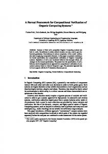
Analyzing these end-to-end effects over several components requires knowing the communication mechanisms of the execution platform that connects these components. Figure 1 illustrates the layered automotive software architecture following the AUTOSAR standard [1] that defines roughly three layers: • the application software: this contains a functional view of software components (SW-Cs) that exchange signals through the mapping-independent virtual function bus (VFB), • the run-time environment (RTE) as a standardized interface for the communication of software components among each other and with the basic software on one particular ECU, and • the basic software (BSW) including the operating system (OS), the communication stack (COM), and input/output and other device drivers (I/O). For the sake of software portability, these layers are developed independent of each other, with hand-over buffers in between. Standardized APIs facilitate easy exchange of parts of the software; OSEK/VDX [10] is established well, and the new AUTOSAR [1] standard borrows many concepts from it. The decoupling buffers (within the RTE) are mostly registers, and the functions can access these registers almost arbitrarily. A second observation is that almost all automotive systems are multi-rate systems. Even if the functional application appears as a single rate system, multiplexing mechanisms in the communication can induce under- and oversampling. To give an example, consider a signal that is updated every 50ms but sent over FlexRay in a frame every 40ms. Such seeming mismatch can result from practical limitations of the used technologies. A FlexRay bus with a
cycle time of 5ms, for instance, only supports frame repetition times of 5ms, 10ms, 20ms, 40ms, 80ms, etc., but not 50ms. In the combination of such over- and under-sampling effects with register communication, some produced signal values are consumed twice while others do not even reach the consumer. This gives raise to the question what “endto-end delay” means. Both mentioned domains chassis and body (and of course, others) make use of multi-rate functions, both rely on correct end-to-end timing, but they essentially differ in the meaning of end-to-end delays. Control systems that continuously drive external actuators shall ensure that these driving signals do not exceed a maximum age. “Data age” is a concept in the heart of control engineering theory. Clearly, if the same signal is consumed twice, the second consumption is critical because the (unchanged) signal at the time of the second consumption is older. In body electronics, the situation can be very different. In the mentioned door lock system, the first arriving signal will command the consuming device to lock the door. Any later signal duplicate can not lock the door “more”. This shows that there exist at least two different semantics of end-to-end timing that have -to the best of our knowledge- not been previously distinguished. In this paper we first review the existing work on end-toend scheduling analysis. In Section 3, we introduce a framework that allows defining end-to-end paths and provides several reachability tests. Based on these, paths of different semantics can be distinguished and their delays can be calculated in the presence of multi-rate register-based communication. In Section 4, we extend this framework to several different end-to-end semantics including the two mentioned already. We discuss the general applicability of the approach and survey possible extensions in Section 5. Finally, we draw our conclusions and point out future research directions.
2
Known End-to-End Analysis
Scheduling analysis of individual components (ECU or bus) has been studied extensively. Numerous approaches to static-priority (SP) scheduling have been proposed that enable analysis of OSEK (preemptive SP or SP with deferred preemption) and CAN systems (non-preemptive SP). Ratemonotonic scheduling [7] was just the start. The response time approaches [5], in particular, became accepted because they provide comprehensive results, especially when complemented by the corresponding Gantt chart views that let engineers understand the details of software execution that lead to the one or the other critical timing situation. TDMA analysis can be applied to FlexRay buses [6]. The abstract
approaches to analyzing SPP, SPDP, SPNP, and TDMA scheduling can be adjusted to cover well the behavior of real-world automotive systems [17]. Compared to the number of single-processor scheduling analysis approaches, end-to-end timing has received far less attention so far. The introduction of task offsets to response time analysis by Tindell [16] has set a mark in real-time systems research. In addition to the significant accuracy increase for systems with offsets (as found in OSEK and CAN schedule tables), the approach also covers event-triggered end-to-end paths through several tasks distributed over several hardware components. The basic idea is to calculate response times of transactions comprised of several chained tasks. Later, the approach was extended in many ways in order to reduce pessimism further, e.g. to dynamic offsets [11] and precedence relations [12, 13]. However, the approach neither regards general multi-rate systems nor register-based communication. It is based on event-triggered activation and FIFO queuing. Richter and Ernst [14] introduced a compositional scheduling model that uses local response time calculation following single-resource approaches such as Tindell’s work [16]. They then characterize the external interaction of these components through event stream models and introduced a set of different event stream interfaces. Chakraborty and Thiele [15] followed another compositional approach based on real-time calculus with local service and arrival curves to calculate delays and backlogs. However, both groups focused mostly on FIFO queuing. Registers in a multi-rate system were not considered deeply so far. Mangeruca, Beneviste, and others [8, 2] recently proposed a relaxation that is based on communication-bysampling (CbS) and also supports multi-rate systems. The approach targets “semantics preservation”, achieved by relaxing the constraints of FIFO communication and to account for under- and over-flow prevention. Their approach can be further reduced into a register model by setting FIFO size to one. The authors propose mechanisms that shall ensure “semantics preservation” by deliberately constraining the way “the consumer must access the buffer” [8]. In a similar way, Matic and Henzinger [9] proposed slight changes to the way task schedules are build during system generation by model-based design tools. Both approaches require that certain platform mechanisms are used in a specific way - the way that preserves the semantics of the communication. Such restrictions compromise to some extent the broad applicability of the approach in practice today. Therefore, we are seeking a general approach that does not restrict the buffer access. In another older publication, Gerber et. al. studied multirate register-based communication [3] without requiring special semantic preservation mechanisms. However, it is
a synthesis approach that cannot analyze system in general. Furthermore, the synthesis requires that task periods can be changed freely, which is very uncommon in automotive design. In another recent publication, Guermazi and George [4] really analyze periodic systems with register communication. They calculate task and communication service response times locally for each involved component or task, and then create the worst-case sequencing of them by composition, thereby considering additional delays at every involved buffer. Unfortunately, the approach assumes “worst-case asynchronicity” for all register accesses and does not account for offsets. In consequence, the results are overly pessimistic and therefore of limited relevance in automotive systems, where OSEK time table offsets and synchronization with FlexRay are key mechanisms to reduce delays. All mentioned publications shed a light on one or the other issue relevant for end-to-end timing analysis. To the best of our knowledge, the differentiation of end-to-end semantics in the presence of multi-rate register communication has not been considered so far, despite its importance in automotive system design (and avionics and other industries). This will be introduced in the next section.
3
End-to-End for Register Edges
Figure 2 shows an example of an end-to-end path through four tasks (t1 , t2 , t3 and t4 ) are three register buffers (r12 , r23 , r34 ). All tasks are activated with different periods (T1 , T2 , T3 , T4 ), so the example is essentially a multi-rate system. T1=40
rin
t1
T2=10
r12
t2
T3=30
r23
t3
T4=20
r34
t4
rout
p=(t1,t2,t3,t4)
Figure 2. Example end to end path Before we start distinguishing the different semantics, we will introduce a set of data-path reachability conditions and provide a calculation framework for end-to-end delays. The actual distinction of several semantics within this framework is introduced in Section 4.
3.1
Delay calculation framework
The scheduling of tasks determines in which order read and write accesses are made to register values, where each individual register access results from one dedicated instance of one dedicated task. Moreover, each specific task
instance will read data from this input registers and write data to its output registers, where they are read by another instance of another task, and so on. Consequently, we can associate the timing of such a “data journey” through a path with a sequence of specific task instances. We will call a specific task instance sequence a timed path tp.
Def. of a Path
a1=1
t1
F
a2=2
t2 C
t3
G E
a3=1 A
t4
B
a4=2
through. However, this information is already exploited in the definition of the timed path, and there exist several ones (see Figure 3). The question is, which timed path is the “right” one? Apparently, only paths shall be considered in which data is actually communicated among the task instances within that timed path. We call such paths valid timed paths. In order to be considered valid, the data must be able to actually pass through the task instances in the described way. Hence, we have to ignore all paths that involve backward jumps (time-travel) as well as forward jumps that are too long (and become overwritten).
D
3.2
Forward Reachability
time
tA
• •
Figure 3. = Several Timed Paths bold: A = (a1,a2,a3,a4) (1,2,1,2) D = (1, 5, 2, 4) Figure 3 illustrates several such sequences for the path of Figure 2. To give an example, the bold arrow denoted A illustrates the task instance sequence −→ tpA = (1, 2, 1, 2)
We start with the backwards jumps as obvious criteria to mark a timed path non-reachable because it would require time travel of data. Clearly, a reading task instance must not be activated before the writing task instance. As an example, the path G in Figure 3 is not reachable, because it contains time-traveling data.
TimeTravel & Waiting critical non-waiting read Æ no valid path
(1) t1
x where tpA i denotes the instance of the ith task in that path. t2 Once, we know the timed path, the actual time of that critical waiting read journey is solely determined by the read access of the first t3 and the write access of the last task instance in that timed t4 path. All intermediate task instances can be ignored. This non-critical read provides a powerful abstraction from the internal schedultime ing. 4. Influence of scheduling on data For the moment, we restrict the analysis to tasks that read• criticalFigure (reader is activated during writer execution): communication in the beginning and write in the end. Most OSEK tasks in – waiting read: valid fact do that (through specific value-copy calls) for reasons – non-waiting: invalid of consistency maintenance. Consequently, the first read • non-critical: valid can be safely bounded to appear no earlier than the activaHowever, this activation time-travel criteria is necessary A tion of the corresponding task instance tp1 , while the last but not yet sufficient to eliminate time travel. Not only write is the termination time of the last task instance tpA 4, the activation time must be considered but also (and more given by the activation time α and its worst-case response importantly) we must check if the tasks instances have a time δ. This response-time of the second instance of task t4 chance to communicate. Figure 4 illustrates three situations is illustrated as a gray bar in the figure. that we must distinguish. The bold gray boxes represent The actual end-to-end path delay ∆ of the given timed task execution and data is read at the left border of the ex−→ path tpA is indicated in Figure 3 and given by: ecution and written at the right border. The thinner light boxes represent task preemption that (in this example) fol−→ A A ∆(tpA ) = αn (tpA ) + δ (tp ) − α (tp ) lows static-priority scheduling. n 1 n n 1 The situations are marked with attributes critical and = α4 (2) + δ4 (2) − α1 (1) (2) waiting. In case of a non-critical read, the writing task inIn this equation, information on the timing of the internal stance has already completed execution when the reading tasks t2 and t3 is not required for calculating the path delay. instance is activated, no time-travel. In the situation of critThis might seem surprising because the timing of the tasks ical waiting read, the reader is activated while the writer is still executing. However, the reader must wait until the t2 and t3 does in fact influence the timing of data that travels
writer completes (because of the priorities), so these two instances can communicate; no time travel. In case of critical, non-waiting read, the reader preempts the writer and starts reading before the writer has written its output. These two instances do not communicate and a timed path containing these instances is not valid; or not reachable.
3.3
Overwrite and Waiting Overwrite Elimination
3.4
Mathematical Framework
We can define a set of simple boolean function that assist in determining forward reachability and overwriting between the ith instance of a writing task tw and the jth instance of a reading task tr . The following boolean function att returns true if “activation time travel” occurs (i.e. when the reader is activated before the writer), and false if it doesn’t: att(tw (i) → tr (j)) = (αr (j) < αw (i))
The more important “critical function” crit determines if (even in case of non-activation time travel) writer and reader overlap in execution:
t1 t2
crit(tw (i) → tr (j)) = (αr (j) < αw (i) + δw (i))
t3 t4 time
(4)
And the waiting function wait determines if (in case of overlapped but not time-traveling execution) the writer finishes first, because the reader has to wait due to its priority: wait(tw (i) → tr (j)) = (p(tr ) < p(tw ))
Figure 5. Data history border
• •
(3)
(5)
additional load mightNow, turn we can combine these to define a boolean funcnon-critical into critical reads; tion forw determining the forward reachability of the two ti+1 must read „newest“ ti (no older) then, the non-waiting ones The instances must not time travel (¬att, Eqn. 3) So far we have considered communication that is uninstances. newest must consider critical non-waiting „create“ new history borders reachable because it represents a backward time-travel. and additionally be either not critical (¬crit, Eqn. 4) or wait
Now we will consider another type of time-traveling that results from overwriting. The fact that data can be overwritten, in particular in the presence of under-sampling, leads to dead ends in timed paths. Figure 5 illustrates this situation. Dead ends are drawn with a dotted line. A new write access of a specific task instance enforces a history border through which no earlier instance of the same task can communicate. History borders are marked with gray curved lines With the above checks, we can eliminate all non-valid timed paths, so only those paths remain, along which communication actually takes place. From these, we can choose the one with the longest delay according to Equation 1. Figure 6 shows that our example contains four valid timed path −−→ with timed path D (tpD ) being the longest.
LONGEST !!!
t1
forw(tw (i) → tr (j)) =
¬att(tw (i) → tr (j)) ∧ (¬crit(tw (i) → tr (j)) ∨ wait(tw (i) → tr (j)))
=
¬ (α(tr (j)) < α(tw (i))) ∧ (¬ (αr (j) < αw (i) + δw (i)) ∨ p(tr ) < p(tw )) (6)
From this forward reachability, we can also detect overwrites. The output of an instance tw (i) is overwritten by instance tw (i + 1) when both instances can forward reach the same reading task instance tr (j). In other words, tw (i) can reach tr (j) if and only if the following function returns true: reach(tw (i) → tr (j)) =
t2 t3 t4
(wait, Eqn. 5):
(forw(tw (i) → tr (j)) ∧ ¬forw(tw (i + 1) → tr (j))) (7)
F A
H
D
time
Figure 6. Maximum Path Delay
• D = (1, 5, 2, 4)
From this reachability between two task instances, we can now define the reachability function for a whole timed path. A timed path is reachable, if and only if every two consecutive task instances within that path are reachable. Y → − reach( tp) = reach(ti (tpi ) → ti+1 (tpi+i )) (8) i=1...n−1
first in
last in input interval
Task A Task B Task C
first out
output interval
last out
a: first Æ first b: first Æ last c: last Æ first d: last Æ last
Figure 7. Example with Task Schedule and Several End-to-End Semantics We finally have to do this for all possible timed paths, and we obtain the set of all reachable timed paths TPreach : → − → − TPreach = { tp ∈ Nn | reach( tp)} (9) Together with Equation 1, we can now determine the maximum latency over all reachable paths: → − → − ∆LL (p) = max{∆( tp) | tp ∈ TPreach } (10) The superscript LL indicates the “last-to-last” semantics which is explained in the next section.
4
Other End-to-End Semantics
In the preceding section, we have identified key properties of data reachability within register communication paths, and we have provided a first end-to-end calculation. This so far presented delay calculation follows the semantics of “maximum data age”. This section introduces extensions that allow covering also other semantics, based on reachability functions introduced above. Generally speaking there are four different semantics possible in an over-/under-sampling situation. These possibilities are illustrated in Figure 7. The input and output intervals illustrate the time span in which input changes have an impact on the delay and output data is actually becoming available. The so far introduced “max age” semantics corresponds to the “last-to-last” paths from that figure. The formulation “last-to-last” refers to the fact that it considers the delay between the last input (that is not overwritten) until the last output (even in case of duplicates). In the next paragraphs, we extend the formal framework to cover also the remaining three semantics.
4.1
Last-to-First
In this case, we are seeking the maximum delay of all non-overwritten (“last”) inputs until the non-duplicate (“first”) output of the path. This is a bit more complex that the above mentioned calculation, because we must ignore all timed paths that lead to later (non-first) duplicates of other paths with the same start instance. With respect to Figure 6, this applies to timed path H and D, which produce duplicate of path A data. Simply speaking, the set of all non-duplicate, reachable timed paths TPfirst is that sub-set of all reachable timed path TPreach for which no timed path exists that shares the same start instance of the first task and has an earlier end instance of the last task. → − TPfirst = { tp ∈ TPreach | − → ¬∃tp0 ∈ TPreach : tp01 = tp1 ∧ tp0n < tpn } (11) The maximum “last-to-first” timed path delay ∆LF is given by: → − → − ∆LF (p) = max{∆( tp) | tp ∈ TPfirst }
4.2
(12)
First-to-Last and First-to-First
So far, we have considered semantics where the last nonoverwritten input is considered, i.e. that input that actually travels through the path. Now, we will consider also inputs that are overwritten. This is important in situations where we are interested in the delay that system needs to react to value changes at the input that can arrive asynchronously
at any time. So we have to include in the calculations an initial “input sampling delay”. This input sampling is often assumed to be the period of the first task of the path, like in [4]. The underlying idea is that new data can “just miss” the read access of the input task and has to wait for the next instance of that input task. While this assumption is correct in single-rate systems without jitter, it produces wrong results in multi-rate systems, because over- and under-sampling introduces internal delay effects that can significantly increase this input delay. To be precise, we have to look backwards to that point in time at which a newly arriving data has the chance to travel through (or reaches) the entire path. When this point is missed, the data will in fact be recognized by the system at the next input task instance, but the whole system will not respond to it until the next fully reachable path, which can start even later. This is illustrated in Figure 7. To determine the actual delay, we have to add to each “last-to-x” path delay the temporal distance to the start of the latest previous “last-to-x” path. Hence, we have to determine the start task instance of the previous reachable “last→ − to-x” path that we will call pred( tp):
This vertical composition makes the approach flexible in two ways:
→ − pred( tp) =
5.3
− → max{m ∈ N | m < tp1 ∧ ∃tp0 ∈ TPreach : tp01 = m} (13) Now, we can calculate the “first-to-last” path delay ∆F L by → − → − → − ∆F L ( tp) = ∆LL ( tp) + α1 (tp1 ) − α1 (pred( tp)) → − → − ∆F L (p) = max{∆F L ( tp) | tp ∈ TPreach }
(14) (15)
and the “first-to-first” path delay ∆F F by: → − → − → − ∆F F ( tp) = ∆LF ( tp) + α1 (tp1 ) − α1 (pred( tp)) → − → − ∆F F (p) = max{∆F F ( tp) | tp ∈ TPfirst }
5
(16) (17)
Properties and Possible Extensions
After introducing the formal framework, we now outline few key properties of the approach.
5.1
Vertical Composition
The proposed end-to-end calculation assumes that a “normal” scheduling analysis of tasks or frames has already been performed. In all formulas, only activation times α and response times δ play a role. No further details of task scheduling are required. In this context, the end-to-end analysis represents a vertical composition since it builds upon previous scheduling analysis results.
• the framework also supports relaxed task models incl. periodic tasks with jitter or burst, and • the framework also supports other schedulers such as TDMA (required for FlexRay analysis), EDF, or round-robin as long as activation models (α) are known and worst-case response times (δ) can be determined.
5.2
Horizontal Composition
Horizontal composition means that we can analyze the end-to-end latency (following the same semantics) of two independent sub-systems, and then combine the sub-system delays into a system delay. We can account for the possible delay between the sub-systems in the same way that we have considered the input sampling delay in Section 4.2.
Practicability Concerns
The sets of timed paths TP, TPreach , and TPfirst are subsets of Nn and therefore generally unbounded. However, with periodic tasks, the number of relevant paths can be bounded to those that start within the first macro-period, i.e. within the least common multiple (LCM) of all involved periods. This is a property already exploited in rate-monotonic scheduling and its offset-aware extensions. With this in mind, the mentioned path sets become bounded. In addition, the number of reachable timed paths within a macro period can not exceed the number of instances of the task with the smallest period. This is intuitive since each such “fastest” task instance can be contained in at most one reachable path. This way, the algorithmic complexity does not grow exponentially, as the set size Nn might suggest, but it grows linearly with the size of the macro period.
5.4
Application in Automotive Systems
Both, the vertical and the horizontal compositionality make the approach applicable to distributed automotive systems with multi-rate, register-based communication, layered software architecture, and a mixture of scheduling concepts. The vertical composition lets us capture well the OSEK, CAN, and FlexRay specific scheduling analysis, and it lets us consider jitter in tasks and driver interrupts. The horizontal composition lets us analyze the end-to-end timing over several ECUs that communicate over CAN and/or FlexRay.
5.5
Relaxed Task Communication
Finally, the approach -again because of its vertical compositionality- can be refined and applied to task models where tasks can read and write data at arbitrary points in time. When these buffer access times are known -as a result from a previous scheduling and communication timing analysis- these results can be used instead of the more abstract activation and response timings in Equations 2 and 3. Equations 4, 5, and 6 are not required anymore and the remaining equations can be used unchanged.
ways. Its vertical compositionality makes the approach applicable to different schedulers (SP, TDMA, RR, and EDF) and for realistic task models, e.g. periodic tasks with jitter or burst, as long as a response-time analysis is available. Its horizontal compositionality makes it applicable to distributed systems with several ECUs and buses, be it synchronous (e.g. with FlexRay) or asynchronous (e.g. with CAN). In addition, the generality of the approach provides opportunities for extensions in several directions, of which we have highlighted a few.
References 5.6
Internal Task State [1] The AUTOSAR Development Partnership. Automotive Open System Architecture (AUTOSAR). URL: http://www.autosar.org, 2003.
Finally, also internal state of tasks can be incorporated. Such internal state could, for instance, turn the task into a FIFO pipeline such that each newly read input data is written to the output one instance later. This is not an artificial example but exists in practice also in automotive systems when so called software component data structures are used. These prevent that two functions that are mapped to the same task can communicate during the execution of the same instance of that task; hence, two task instances are needed to let these function communicate. The end-to-end delay calculation framework supports such cases, we simply have to put the task into the path twice, and all other calculations apply.
6
Conclusion
In this paper, we have introduced a formal framework for defining end-to-end delays in the presence of multirate, register-based systems. Having such a framework is a prerequisite for analyzing end-to-end delays in automotive software systems because these systems are inherently multi-rate and use mostly register communication. In contrast to previous work on end-to-end analysis, our approach presents a general solution that does not constrain the way, buffers are accessed. We consider this an important requirement for the industrial acceptance of scheduling analysis. A second key finding of this work is the existence of several different semantics (meanings) of end-to-end delay that must be carefully distinguished from one another. The “max data age” (or “last-to-last”) semantics is needed for delay calculation in control engineering, while the “first reaction” (or “first-to-first”) semantics is the first choice for body electronics where “button-to-action” delays are critical. To the best of our knowledge, previous work on end-toend analysis has ignored the existence of different end-toend semantics. We have further shown that the proposed calculation of the delays is flexibly applicable and extensible in many
[2] A. Benveniste, P. Caspi, M. di Natale, C. Pinello, A. Sangiovanni-Vincentelli, and S. Tripakis. Loosely time-triggered architectures based on communicationby-sampling. In EMSOFT ’07: Proceedings of the 7th ACM & IEEE international conference on Embedded software, pages 231–239, New York, NY, USA, 2007. ACM. [3] R. Gerber, S. Hong, and M. Saksena. Guaranteeing end-to-end timing constraints by calibrating intermediate processes. In IEEE Real-Time Systems Symposium, pages 192–203, December 1994. [4] R. Guermazi and L. George. Worst case end-to-end response times of periodic tasks with an AUTOSAR/FlexRay infrastructure. In 7th International Workshop on Real-Time Networks RTN’08, 2008. [5] M. Joseph and P. Pandya. Finding response times in a real-time system. The Computer Journal, 29(5):390–395, 1986. [6] H. Kopetz and G. Gruensteidl. TTP - a time-triggered protocol for fault-tolerant computing. In Proceedings 23rd International Symposium on Fault-Tolerant Computing, pages 524–532, 1993. [7] C. L. Liu and J. W. Layland. Scheduling algorithms for multiprogramming in a hard-real-time environment. Journal of the ACM, 20(1):46–61, 1973. [8] L. Mangeruca, M. Baleani, A. Ferrari, and A. Sangiovanni-Vincentelli. Semantics-preserving design of embedded control software from synchronous models. IEEE Trans. Software Eng., 33(8):497–509, 2007. [9] S. Matic and T. A. Henzinger. Trading end-to-end latency for composability. In RTSS ’05: Proceedings of the 26th IEEE International Real-Time Systems Symposium, pages 99–110, Washington, DC, USA, 2005. IEEE Computer Society. [10] OSEK Steering Committee. OSEK Open systems and the corresponding interfaces for automotive electronics. http://www.osek-vdx.org/. [11] J. C. Palencia and M. G. Harbour. Schedulability analysis for tasks with static and dynamic offsets. In Proceedings of the IEEE Real-Time Systems Symposium, page 26. IEEE Computer Society, 1998. [12] J. C. Palencia and M. G. Harbour. Exploiting precedence relations in the schedulability analysis of distributed real-time systems. In Proceedings of the IEEE Real-Time Systems Symposium, pages 328–399. IEEE Computer Society, 1999. [13] O. Redell. Accounting for precedence constraints in the analysis of tree-shaped transactions in distributed real time systems. Technical report, Department of Machine Design, KTH Royal Institute of Technology, Sweden, 2003. [14] K. Richter, D. Ziegenbein, M. Jersak, and R. Ernst. Model composition for scheduling analysis in platform design. In Proceeding 39th Design Automation Conference, New Orleans, USA, June 2002. [15] L. Thiele, S. Chakraborty, and M. Naedele. Real-time calculus for scheduling hard real-time systems. In Proceedings International Symposium on Circuits and Systems (ISCAS), Geneva, Switzerland, 2000. [16] K. Tindell. Adding time-offsets to schedulability analysis. Technical Report YCS 221, Department of Computer Science, University of York, UK, 1994. [17] K. Tindell, H. Kopetz, F. Wolf, and R. Ernst. Safe automotive software development. In Design, Automation and Test in Europe Conference, pages 616–612, Munich, Germany, March 2003.