Aug 27, 2003 - Buyers sequentially initiate market-sessions by submitting RFQs (Request for. Quote) to the broker. In real-life marketplaces, each buyer is at ...
A Computational Approach to Compare Information Revelation Policies Amy Greenwald, Karthik Kannan, Ramayya Krishnan August 27, 2003
Abstract Revelation policies in an e-marketplace differ in terms of the level of competitive information disseminated to participating sellers. Since sellers who repeatedly compete against one another, learn based on the information revealed and alter their future bidding behavior, revelation policies affect the welfare parameters - consumer surplus, producer surplus and social welfare - of the market. Although, different revelation policies are adopted in several traditional and web-based marketplaces, prior work has not studied the implications of these policies on the performance of a market. In this paper, we study and compare a set of revelation policies using a computational marketplace. Specifically, we study this in the context of a reverse-market where each seller’s decision problem of choosing an optimal bid is modeled as an MDP (Markov Decision Process). Results and analysis presented in this paper are based on market sessions executed using the computational marketplace. The computational model, which employs a machine-learning technique proposed in this paper, ties the simulation results to that developed using the game-theoretic models. In addition to this, the computational model allows us to relax assumptions of the game-theoretic models and study the problem under a more realistic scenario. Insights gained from this paper will be useful in guiding the buyer in choosing the appropriate policy
1
1 Introduction The motivation for this paper comes from a real-life electronic marketplace. FreeMarkets1 , a webbased reverse marketplace, initiates market-sessions or periods at the request of buyers. The marketplace includes geographically distributed sellers which face uncertainty both about the number of competitors (referred to as market structure uncertainty) and their opponents’ cost structure. Their ability to overcome these uncertainties is dependent on the “market transparency” scheme, or the information revelation policy, choice made by the buyer. An information revelation policy dictates the information about bids – winning bids, number of bidders etc. – that are revealed to geographically dispersed sellers in the beginning, in the middle and at the end of a market-session. At one end of the spectrum of available policies, the buyer can choose to accept sealed bids and notify its decision to each seller individually. Under this policy, no other competitive information is revealed to the sellers. At the other end of the spectrum, the buyer can choose a revelation policy that allows the sellers to observe all bids submitted by their opponents in real-time. Under this policy, all competitive information is revealed. Over the course of multiple market-sessions, the revelation policy affects what sellers learn, how they bid in the future and the overall performance of the market. To our knowledge, this important problem – the impact of these revelation policies – has not been studied in any prior work. This leaves little guidance for the buyer to choose the appropriate policy. One of the reasons that this problem has not been studied thus far could be that these diverse revelation policies were not feasible to implement without the Internet or information technologies. Comparing revelation policies is relevant only in the context of a web-based marketplace, because of the unique nature of the web in controlling the transparency to competition. For example, 1
http://www.freemarkets.com
1
revelation policies such as the one where sellers are informed about their rank relative to other competitors are possible only because of the computational power available. To investigate the implication of such policies, we began attacking the relevant sub-problems analytically. In our earlier paper, Arora et al. (2002), we analytically compare the expected price paid by the buyer in two such revelation policies. This comparison is executed in a framework where sellers are uncertain only about their market structure. A similar comparison is executed in Kannan & Krishnan (2003), in a framework where sellers are uncertain only about their opponent’s cost structure. More details about these results are presented in Section 3. But the key point from these two papers is: when combining both types of uncertainties – market structure uncertainty and cost structure uncertainty – we demonstrate that the comparison becomes analytically intractable. We overcome the difficulty in this paper by computationally studying the effect of revelation policies in a framework where both types of uncertainties can be combined. For this paper, we consider the following two policies which were employed in both Arora et al. (2002) and Kannan & Krishnan (2003): 1. Complete Information Setting (CIS): At the end of a reverse-auction, all quotes are revealed to all bidding sellers. 2. Incomplete Information Setting (IIS): At the end of a reverse-auction, only the winner’s bid is revealed to all bidding sellers. These are two of the many policies available to a buyer in reverse-markets hosted by Freemarkets. We chose to study these specific policies because they are commonly adopted in both traditional marketplaces and electronic marketplaces (Thomas (1996)). The impact of these policies is explained for each type of uncertainty while describing the problem context in Section 2. 2
Although our work is motivated by a real-world electronic marketplace hosted by Freemarkets, its applicability is broader. Results generated in this paper are applicable to any reverse-market setting that can create these different information regimes. The objective of this study is to understand the bidding behavior of sellers under
CIS
and
IIS in
a framework closer to reality i.e., a
framework involving both types of uncertainties. The intuition gained is intended to guide the buyer in choosing the appropriate policy. The paper is organized in the following manner. Following the problem context description in Section 2, we review the literature most relevant to this topic in Section 3 and position this paper with respect to prior work. After that, we describe the computational model developed in Section 4. Results from executing market-sessions on the computational marketplace are presented in Section 5. Finally in Section 6, we conclude.
2
Problem Context
In our reverse marketplace, there are three types of participants – buyers, the broker (the marketmaker) and sellers. Buyers sequentially initiate market-sessions by submitting RFQs (Request for Quote) to the broker. In real-life marketplaces, each buyer is at the liberty of choosing its desired revelation policy whereas in this paper, the information revelation policy is an exogenous variable, the effect of which we study. The broker acts as an intermediary for the marketplace with Nl low-cost sellers and Nh highcost sellers. A low-cost seller incurs zero marginal cost of production whereas a high-cost seller incurs an exogenous ch . Only a subset of all these sellers bid in each market-session. Participation is assumed to be a random process determined by an exogenous parameter – θl or θh . θl is the
3
exogenous participation probability for the low-cost type and θh is that for the high-cost type. In this computational marketplace2 , the task of deciding about seller participation is delegated to the broker. The broker samples a uniform distribution for each seller for each market-session and decides participation for that seller. Although sellers know the values of θl and θh , the realized values of the participation probabilities are not known3 . In this manner, we capture the uncertainty faced by each seller. Each participating seller, i, bids a price, pi ∈ [0, 100]. The price bid is dependent on the following: information revelation policy adopted in the marketplace, its belief about being a monopolist and its belief about being the only seller of its cost-type in the reverse-market. After receiving all bids, the buyer chooses the lowest priced seller as the winner (ties are broken randomly) and awards the contract. The buyer’s decision problem is
arg min pj j
(1)
While developing the product, the winner incurs a cost corresponding to its cost type. The built product is delivered to the buyer who in turn, remunerates the winner. This point corresponds to the end of one market-session. At the end of this market-session, information about the bids submitted is revealed, according to the revelation policy adopted in the marketplace. The information 2 An exogenous participation probability value is assumed for simplicity. Typically, the market-maker sends invitations to sellers. The set of sellers invited to participate may vary depending on what the incentives are for the market-maker. Incentives for some market-makers may be aligned with consumer surplus (e.g. Freemarkets). Other market-makers may have an incentive to maximize social welfare (e.g. marketplaces such as Transora, ForestExpress where the marketplace is owned by consortia of both buyers and sellers). After receiving the invitation, a seller may choose to accept or reject the invitation. Its decision could be based on: production capacity constraints, expected profits from participation etc. The outcome of this series of complex processes is assumed to be captured by the variable a in our model. 3 For example when θl = 12 , sellers know that nature tosses a coin for each low-cost seller and allows that seller to participate only if the outcome is a head. But sellers do not know if the outcome was a head or a tail when nature tossed a coin to decide whether or not to permit one of the low-cost opponents to participate in that market-session.
4
Beginning of a market-session At the end of a market-session Beginning of the next market -session
Impact on Market Structure Uncertainty
Impact on Cost Structure Uncertainty
Complete Information Setting (CIS) Uncertain All bids are revealed All sellers are aware of market structure
– When no other price bid is observed, seller learns that it is a monopolist. – Otherwise, it learns about its competitor. –When a price lower than ch is bid by an opponent, a seller learns about the low-cost opponent.
– Otherwise, it is not sure. It could be that the low-cost opponent faked.
Incomplete Information Setting (IIS) Uncertain Only winner’s bid revealed – Losing Seller is aware of the market structure. – Winner from the first marketsession continues to be uncertain. – When a seller loses, it learns about the existence of competition. – But if it wins, it learns nothing about market structure. – When a seller loses and observes a price lower than ch bid by the winner, it learns about the winner’s cost structure. If it observes the winner’s bid price to be greater than ch , it is not sure if any of its opponents is a low-cost type. – But if it wins, it learns nothing about cost structure.
Table 1: Information Revealed under each Policy
revealed allows sellers to learn about the nature of their competition for future market-sessions. Table 1 describes
CIS
and
IIS
policies in detail. The table also provides a descriptive explanation
of the impact of these policies on each type of uncertainty. A similar process is repeated when the next buyer initiates a new market-session. The key difference between the first and the second market-sessions is that with a certain exogenous probability k, the same set of sellers which participated in the first market-session bid in the second market-session also. With a probability of 1 − k, a new set of sellers bid in the second marketsession. The value of k determines the participation correlation across market-sessions, , ρ.4 4
ρ=
k2 (k2 +(1−k)2 )
5
When ρ = 0, each market-session is entirely independent of the other and there is no value for the sellers to learn across market-sessions. But when ρ = 1, the value from learning about the competitive nature is very high. In reality, ρ is neither 0 nor 1 but some in between5 . We intend to study the impact of these revelation policies for different values of ρ by controlling k. The reverse-auction process is iterated T times i.e., we simulate the arrival of T buyers to the e-marketplace. We are interested in studying the impact of varying T on the expected prices paid by each of the T buyers. As noted by Engelbrecht-Wiggans (2001), analyzing the impact of the number of periods is important in a multi-period game (or a multi-period reverse-auction setting). The impacts of these parameters – ρ and T – are studied by using the computational marketplace described in Section 4. The need for such a computational model is explained in the following section where we review the relevant literature.
3 Literature Review Revelation policies in financial markets are referred to as “Trade-Transparencies” by “Market Micro-Structure” literature. Depending on whether information about outstanding orders or completed orders are revealed, these policies are respectively called “pre-trade transparency” or “posttrade transparency”. Information revealed under these transparency schemes includes the number of securities purchased/sought, price and other details of the limit order. A number of papers have studied the impact of these trade transparencies. In this section, we review a few of them and differentiate our work from prior work done in this area. We begin with the literature on post-trade transparency schemes. Flood et al. (1999) use an experimental study resembling a foreign exchange market – multiple dealer market with inter-dealer 5
Based on anecdotal evidence from Freemarkets Inc.
6
trading – to study the impact of post-trade transparency policies. They show that opaque markets are more efficient but have higher spreads than transparent ones. This result contradicts Bloomfield & O’Hara (1999) who also use experimental economics. Bloomfield & O’Hara (1999) find that in a regular market without inter-dealer trading, post-trade transparency improves informational efficiency but with higher bid-ask spreads. Next, we review the literature on pre-trade transparencies. Madhavan et al. (1999) and Anand & Weaver (2001) use data from the Toronto Stock Exchange and demonstrate that opaque markets lead to lesser efficiency. This again contradicts with Boehmer et al. (2002) who use data from the New York Stock Exchange. Note that these results are not applicable to electronic reverse-markets because of structural differences between the two types of markets. Typically, financial exchanges are double-sided auctions6 whereas electronic reverse-markets are single-sided auctions. Information revealed in a double-sided auction not only affects the behavior of sellers but also that of buyers. In a singlesided reverse-auction, information revealed affects the behavior of sellers only. These differences make revelation-policy-comparisons in our procurement e-marketplace context different from that in financial markets. To our knowledge, revelation policies in single-sided auctions have been studied only by Thomas (1996), Koppius & van Heck (2002), Arora et al. (2002) and Kannan & Krishnan (2003). Thomas (1996) compares CIS and IIS in a framework with two sellers, where each seller is certain about the presence of its opponent but uncertain about its opponents’ cost structure. The model assumes that each seller faces an opponent which is a high-cost type with a probability of 12 . Using this model, he demonstrates that
CIS
generates higher savings for the buyer than
IIS .
Our other
paper, Kannan & Krishnan (2003), further generalizes the model by Thomas (1996). We defer the 6
The only financial market which operates as a single-sided auction is the primary bond market (e.g. US Treasury Bills). Even in these bond markets, the standard policy is to reveal the winner’s bid and the quantity purchased.
7
discussion on Kannan & Krishnan (2003) to later part of this section. Koppius & van Heck (2002) use experimental data to compare revelation policies on bidders’ profits in a multi-attribute auction setting. They show that the setting that creates the least level of uncertainty for bidders generates the highest profit for them. In their paper, bidders face the following types of uncertainties – uncertainty about the valuation that the buyer places on each attribute and uncertainty about their opponents’ cost structure. Our present paper is different from both Koppius & van Heck (2002) and Thomas (1996) in its focus. In our present paper, we study the effect of information revelation policies in a framework where sellers face uncertainty both about the market structure and opponent’s cost type. A special case of this framework is analyzed in our earlier papers, Arora et al. (2002) and Kannan & Krishnan (2003), where each type of uncertainty is considered separately. Each of our earlier papers employs a two-period game-theoretic model for the problem context described below. Two buyers arrive at an e-marketplace and initiate two reverse-auction periods. In each period, participating sellers simultaneously bid prices and the lowest price wins. In both frameworks, we assume that the same set of sellers participate in both periods. Stated differently, the participation correlation across market-sessions is unity. We use this set-up to study the impact of the revelation policy choice made by the first buyer. The only difference between the two frameworks is the type of uncertainty that sellers face. In Arora et al. (2002), all sellers have identical cost-structures but they are uncertain about the number of opponents in the reverse-market – market structure uncertainty. In Kannan & Krishnan (2003), there are two low-cost sellers and other high-cost sellers in the reverse-market. Each seller is aware of the total number of opponents it is facing but it is uncertain about the presence of low-cost opponents in the reverse-market. These models relate to our current work in the following manner: Arora et al. (2002) corresponds to the 8
setting T = 2, k = 1 and Nh = 0 and Kannan & Krishnan (2003) corresponds to T = 2, k = 1 and Nl = 2. Using these models, the expected prices paid by the buyer in CIS and in IIS are compared. In Arora et al. (2002) i.e., the framework with market structure uncertainty, we could not compute the analytical expression for the equilibrium in CIS
generates higher savings for the buyer than
IIS
IIS .
Despite this, we demonstrate that
just by using the lower bounds for
intuition for this result is as follows. Recall that at the end of the first period in
CIS,
IIS .
The
all bids are
revealed, allowing sellers to learn about their market-structure independent of whether they won the first period or not. In contrast, only the winner’s bid is revealed at the end of the first period in IIS .
This implies that all sellers except the first-period winner are aware of the presence of at least
one competitor. But the first-period winner continues to be uncertain about the market structure even in the second period. In order to avoid this uncertainty in the second period, sellers are willing to pay in the first period. They pay so by bidding a higher first period price thus, leading to a higher expected price paid by the buyer in IIS than in CIS. In Kannan & Krishnan (2003), low-cost sellers may have an incentive to fake their cost structure when all bids are revealed in
CIS.
This faking behavior leads to a higher expected price paid
by the buyer in CIS than in IIS. We demonstrate this result by performing the analysis numerically. The need for such an analysis arises because the comparison becomes analytically intractable even under a simplistic setting with a fixed number of sellers. When uncertainty about the number of sellers is introduced, the problem becomes more complex thus, making a case for the computational model (Kannan & Krishnan (2003)). The additional benefit of a computational approach is that one can relax the following restrictive assumptions that are needed for the game-theoretic models and study the impact of these parameters: • The Number of Periods: Only a two period game is studied in the game-theoretic models. In 9
Assumptions Uncertainty about the number of competitors Uncertainty about the cost-type Combining both types of uncertainty Number of sellers
Number of Periods Correlation across periods Participation Probability
Arora et al. (2002) Yes
Kannan & Krishnan (2003) No
Current Paper Yes
No
Yes
Yes
No
No
Yes
n identical sellers M competitors including (Greenwald et al. (2002) n low-cost sellers. proves this) (Kannan (2003) proves this) 2 2 Perfect Perfect (i.e., correlation = 1) (i.e., correlation = 1) Exogenous Exogenous
any distribution of cost-types
any any exogenous value Exogenous
Table 2: Assumptions Made in the Chapters
reality, buyers arrive at the reverse-auction sequentially, initiating each period. So, the game is a multi-period game. • Participation Correlation: Participation correlation across the two periods was assumed to be unity in the game-theoretic models. Stated differently, the same set of sellers that participated in the first period are assumed to continue in future periods also. Based on the anecdotal evidence from Freemarkets, we find that although the correlation is high, it is not unity. Table 2 summarizes the assumptions that can be relaxed in our current paper relative to those in Arora et al. (2002) and Kannan & Krishnan (2003). The computational model adopted in this paper is described below.
10
4 Computational Model In this computational marketplace, software agents are used to mimic the broker, buyers and sellers. From the problem context description in Section 2, it is straightforward to design software agents that mimic the behavior of buyers and the broker. But the optimal bidding behavior of sellers is unknown and so, instead of modeling the bidding behavior, we provide a framework for the “seller-agents” to learn.
4.1 Learning Model The task for any seller, i, is to choose an optimal bid and based on the outcome of the bid, learn to bid in future market-sessions. For this decision-problem, if we knew the relationships between the different parameters, we can employ na¨ive learning models such as Regression, ID3, KNN (kNearest Neighbor) and allow the sellers to learn the weights for the decision-variables. But in our case, the model cannot be completely specified and so the need for a “model-free” approach e.g.. Markov Decision Process (MDP) and Partially Observable Markov Decision Process (POMDP). The factors (or states of the Markov Model) that drive the bidding behavior in our model are: the realized probability value7 of being a monopolist, the realized probability value of being the only seller of its cost type and the current period – one of the T periods. By design, these states are unobservable and the framework corresponds to a POMDP model (Kaelbling et al. (1996)). However, the learning techniques for POMDP are still in the preliminary stages of research and therefore, we model this process as an MDP. The state-space for our MDP framework are – belief about being the only seller of its own cost type (discretized for finiteness of the state-space), belief about being the only seller in the market 7
Outcome of the coin toss described in Footnote 3
11
(discretized for the finiteness of the state-space), the current period – one of the T periods – and finally, whether or not it acted like a low-cost type by bidding a price lower than ch , the high-cost type’s cost, in the earlier period. The last dimension accounts for the knowledge gained by the seller while it fakes its cost-structure. The action chosen by the seller – the price bid – affects how the state-space transitions. If the price bid is pi and the state-space transitions from S to S 0 , the reward (profit or loss) function is: pi − ci
if i wins
0
if i loses
pi RS→S 0 =
In our model, sellers can bid discrete prices only i.e., pi ∈ {10, 20, . . . , 100}. The optimization model used by the seller, given that the seller is in state S, is:
max Q(S, pi )
(2)
pi
where "
Q(S, pi ) =
X
ΩS→S 0
# pi RS→S 0
S0
Q(S + max 0 pi
0
, p0i )
(3)
ΩS→S 0 is the transition probability from state S to S 0 that the environment controls. The beliefs which are a component of the state-space are computed by each seller based on its observation. If bmono represents the belief held by a low-cost seller about being a monopolist, bcost represents the belief held by it about being the only low-cost seller in the reverse-market and M represents the number of market-sessions that it participated in, then beliefs are computed by that seller in the following manner:
12
• Independent of
CIS
or
IIS ,
if it is the first market-session or if the seller participates in a
particular market-session but did not participate in the previous market-session, then:
bmono = (1 − θl )(Nl −1) (1 − θh )(Nh −1) bcost = (1 − θl )(Nl −1)
• Among all the bid prices revealed in
let pj be the lowest bid in the reverse-market
CIS,
excluding its own bid. – if pj < ch
bmono = 0 bcost = 0
– if pj > ch
�
bmono = (1 − θl )(Nl −1) (1 − θh )(Nh −1) (1 − k) + k �
bcost = (1 − θl )(Nl −1) (1 − k) + k
M Mhi
M Mhi
�
�
where Mhi is the number of previous market-sessions, the seller observed a price pj > ch . – But if did not observe any other bid in the reverse-market, then
bmono = (1 − θl )(Nl −1) (1 − θh )(Nh −1) (1 − k) + k 13
bcost = (1 − θl )(Nl −1) (1 − k) + k
• In
IIS ,
if pj is the best price bid that is revealed to all sellers and pi is the bid submitted by
that particular seller – If that seller won the market-session, then pj = pi . Then,
bmono bcost
M = (1 − θl ) (1 − θh ) (1 − k) + k Wpi ! M = (1 − θl )(Nl −1) (1 − k) + k Wpi (Nl −1)
!
(Nh −1)
where Wpj is the number of previous market-sessions, the seller won by bidding pj . – if it lost the market-session and pj < ch , then
bmono = 0 bcost = 0
– if it lost the market-session but observes pj > ch , then
bmono bcost
M = (1 − θl ) (1 − θh ) (1 − k) + k Lpi ! M = (1 − θl )(Nl −1) (1 − k) + k Lpi (Nl −1)
!
(Nh −1)
where Lpi is the number of previous market-sessions the seller lost by bidding pi . In a similar manner, each high-cost seller computes its beliefs. In this framework, the recursive optimization function in equation 2 can be solved analytically 14
Input: Cost c ; c = ch , if seller is high cost type. Similarly c = 0, if low-cost type. Initialize Q(S, pi ) = pi − c ∀S ∀pi ; Stores Q-values Initialize N (S, pi ) = 10 ∀S ∀pi ; Keeps track of the number of iterations Repeat (for each market-session) Initialize S Choose action pi from S using Ratio-Q policy Take action pi , observe R, S 0
[(R−c)+maxp0 Q(S 0 ,p0i )−Q(S,pi )]
Q(S, pi ) ← Q(S, pi ) + N (S, pi ) ← N (S, pi ) + 1 S ← S0 Until End of market-sessions Ratio-Q policy: Given state S
i
N (S,pi )
Qmin = min Q(S, p) ∀p Qmax = max Q(S, p) ∀p e
Q(S,pi )−Qmin Qmax −Qmin Q(S,p)−Qmin e Qmax −Qmin p
choose action pi with probability P
Figure 1: Ratio-Q Algorithm.
if the analytic expression for the transition probabilities, ΩS→S 0 , are known. In fact, one can compute the analytical expression for ΩS→S 0 for ρ = 1 and T = 2 when each type of uncertainty – uncertainty about market structure or uncertainty about their opponents’ cost structure – is considered separately. Such solutions correspond to the game-theoretic models of Arora et al. (2002) and Kannan & Krishnan (2003). But for different values of ρ or T or when both types of uncertainties are combined, computing transition probabilities becomes analytically intractable. In such a case, Reinforcement-Learning algorithms similar to those described in Sutton & Barto (1998) need to be used for solving the recursive equation. The only constraint that the learning algorithm has is that it should be able to identify “mixed-strategy” equilibria. This is important because results from Arora et al. (2002) and Kannan & Krishnan (2003), although for a specific setting, indicate the existence of such
15
Setting Market Structure Uncertainty (Arora et al. (2002))
Cost Structure Uncertainty (Kannan (2003))
First Period Game
Complete Information Setting (CIS) Mixed strategy equilibrium cdf of bid distribution FCIS (p) = 1 − (1−p)(1−a) (p−c)a
Second Period Game
If both sellers exist, they bid p = 0. If one sellers exists, it bids p = 1.
First Period Game
Separating equilibrium is similar to FCIS (p) for low a. Semi-pooling equilibrium for high a. If one seller faked, only a mixed equilibrium exists. Otherwise only a pure equilibrium exists.
Second Period Game
Incomplete Information Setting (IIS) Mixed strategy equilibrium is a solution to a lograthmic equation. First period winner’s distribution 0 (1−c) Fw (p) = 1 − x(p−c) First period loser’s distribution (1−p)x0 Fl (p) = 1 − (p−c)(1−x 0) Mixed strategy equilibrium is a solution to a lograthmic equation. First period winner’s distribution 0 (1−c) Fw (p) = 1 − x(p−c) First period loser’s distribution (1−p)x0 Fl (p) = 1 − (p−c)(1−x 0)
Table 3: Results from the previous papers. Note x0 is the belief held by the first period winner for the second period game.
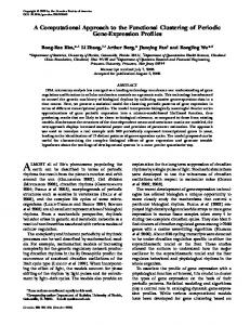
mixed strategy equilibria in this framework (the equilibria are shown in table 3). Standard Qlearning algorithm fails to identify them well. In contrast, a variant of Q-learning algorithm that we developed, Ratio-Q (the algorithm is shown in Figure 1), performs very well. We compare the closeness between the predicted distribution and the empirical bid distribution identified by sellers adopting the algorithm for a specific setting. Specifically, we set Nl = 2, θl = 0.35, Nh = 0 and T = 1 in our problem context description i.e., we consider a single-period game with two low-cost sellers where each seller is uncertain about the participation of its opponent. The probability that each seller observes its opponent is the θl . In this game, the bidding behavior of the sellers can be computed game-theoretically. The 16
Figure 2: Comparing the empirical bid distribution of sellers using Q-Learning Algorithm and the predicted distribution.
Figure 3: Comparing the empirical bid distribution of sellers using Ratio-Q Algorithm and the predicted distribution.
equilibrium is a mixed strategy one, whose cumulative density function (cdf) is:
F (p) = 1 −
θl (1 − p) (1 − θl )p
To compare the closeness of the empirical bid distributions to the predicted distribution, we set-up these parameters in our computational marketplace and execute two sets of 100, 000 marketsessions. In the first set, the sellers were embedded with the standard Q-Learning algorithm. In the second set, sellers were embedded with the Ratio-Q Algorithm. Figure 2 shows the empirical bid distributions of sellers using Q-learning algorithm, and the predicted bid distribution from the game-theoretic model. Similarly, Figure 3 shows the bid distribution for Ratio-Q algorithm and the predicted result. The closeness of each distribution to the predicted values is evaluated using a simple non-parametric test metric – Kolmogorov-Smirnov (K-S) distance. This distance measure is about 0.35 between the empirical distribution with Q-learning algorithm and the predicted values. In contrast, the distance measure is about 0.05 between the empirical distribution with Ratio-Q and the predicted values. Observe that Ratio-Q performs significantly better than the standard
17
Q-learning algorithm8 . We employ this Ratio-Q algorithm in our computational marketplace to execute market-sessions. Results based on data collected from these market-sessions are presented in the following section.
5
Results
Recall that we are interested in understanding how the expected prices paid by the buyer in CIS and in IIS are affected by variations in ρ and T when each type of uncertainty is considered separately. Further, we are also interested in understanding how
CIS
and
IIS
compare when both types of
uncertainties are considered together. We present our hypotheses in section 5.1. Following that in section 5.2, we validate those hypotheses, using data collected from market-sessions executed on our computational marketplace.
5.1 Hypotheses Participation Correlation, ρ, is an important factor which determines how much sellers value learning across market-sessions. The value that sellers obtain from learning is the highest when ρ = 1 i.e., the exact same set of sellers repeatedly participate across market-sessions. At the other extreme, when ρ = 0 i.e., each market-session is independent of the other, there is no value in learning. We know that the expected price paid by the buyer in CIS is lower than in IIS when ρ = 1 under market-structure uncertainty (Arora et al. (2002)). As ρ decreases, the value of learning decreases. This implies that sellers in
IIS
have lesser incentives to increase their first period price
in order to learn their market-structure. So, 8
We also compared these performance under the settings corresponding to papers Arora et al. (2002) and Kannan & Krishnan (2003) and observed that Ratio-Q performs significantly better than standard Q-learning.
18
Hypothesis 5.1 As correlation decreases, the performances of CIS and IIS will tend to be similar when sellers face uncertainty about market structure. Similarly, results presented in Kannan & Krishnan (2003) are valid when uncertainty about opponents’ cost structure is considered separately at ρ = 1. For reasons similar to that presented in the previous hypothesis, we expect the following: Hypothesis 5.2 When sellers face uncertainty about their opponents’ cost structure, the expected price paid by the buyer in CIS and in IIS will tend to be similar as correlation decreases. In multi-period games (reverse-auctions), the number of periods is an important factor dictating the bidding behavior (Engelbrecht-Wiggans (2001)). Under market structure uncertainty, recall that sellers in CIS learn about their market structure at the end of each market-session. Since their learning is independent of the outcome of the market-session, their bidding behavior is not altered. But in
IIS ,
only the winner’s bid is revealed to all participating sellers. So the value that sellers
obtain from losing initial market-sessions is higher as T increases and therefore, we expect the following Hypothesis 5.3 When sellers face uncertainty about market-structure, the difference between the expected prices paid by the buyer in IIS and CIS will increase as T increases. For similar reasons, we hypothesize a similar behavior under cost uncertainty. Hypothesis 5.4 When sellers face uncertainty about their opponents’ cost-structure, the difference between the expected prices paid by the buyer in IIS and CIS will increase as T increases. Now let us focus on combining both these types of uncertainties. It is interesting to observe whether or not CIS is better than IIS. We hypothesize the following:
19
Hypothesis 5.5 When sellers face both types of uncertainties, the expected price paid by the buyer will be higher in IIS than in CIS. The intuition for this result is that the expected price paid by the buyer is lower in CIS than in IIS
(Arora et al. (2002)) when market structure uncertainty is considered separately. Under cost-
structure uncertainty, the expected prices are higher in CIS than in IIS but only for very high values of θl (Kannan & Krishnan (2003). So when combining both these types of uncertainties, we expect the effect of market structure uncertainty to override the effect of uncertainty about opponents’ cost structure.
5.2 Hypothesis Validation We intend to validate these hypotheses by using data collected from market-sessions executed on the computational marketplace. Parameters for this computational model are set similar to a coal reverse-marketplace. Typically, there about 12-15 sellers who can provide coal and out of these, about 3 to 4 participate in each market-session9 . We replicate this by setting Nl = 5, Nh = 6, θl = 0.3, θh = 0.3 and ch = 100 in our computational model. When we deal with just marketstructure uncertainty, participating sellers are of the same type and no uncertainty about opponents’ cost is assumed to exist. Specifically, only the low-cost sellers were assumed to participate. When we model uncertainty about opponents’ cost structure, it is assumed that the uncertainty about the number of competitors does not exist and we retain the number of competitors to 6. For each (ρ, T ) pair, we simulated 200,000 executions on the computational marketplace and the results based on the data collected are summarized below. 9
Based on personal communication with Freemarkets Inc.
20
Complete Information Setting (CIS) 1st Buyer 2nd Buyer ρ = 1.0 29.92 (0.16) 45.35 (0.21) ρ = 0.75 30.12 (0.14) 40.66 (0.18) ρ = 0.5 30.03 (0.16) 37.26 (0.15)
Incomplete Information Setting (IIS) 1st Buyer 2nd Buyer 65.12 (0.17) 47.86 (0.28) 57.35 (0.15) 42.29 (0.25) 48.92 (0.19) 38.06 (0.21)
Table 4: The effect of variation of ρ on the expected price paid by the buyer when sellers are uncertain about their market structure. Standard Deviation shown in parenthesis. Complete Information Setting (CIS) st 1 Buyer 2nd Buyer ρ=1 61.62 (0.26) 48.75 (0.24) ρ = 0.75 55.24 (0.27) 43.28 (0.21) ρ = 0.5 47.53 (0.15) 37.26 (0.22)
Incomplete Information Setting (IIS) st 1 Buyer 2nd Buyer 63.27 (0.13) 46.01 (0.28) 56.54 (0.14) 42.87 (0.27) 49.10 (0.13) 38.38 (0.27)
Table 5: The effect of variation of ρ on the expected price paid by the buyer when sellers face uncertainty about their opponent’s cost structure. Standard Deviation shown in parenthesis.
5.2.1
Testing Hypothesis 5.1
For this analysis, we set T = 2 and executed market-sessions for different values of ρ. Table 4 shows the variation of the expected price paid by the buyer as ρ changes under market structure uncertainty. First, notice that the expected price paid by the buyer is significantly (statistically significant at the 5% level) higher in IIS than in CIS when ρ = 1. This matches the result demonstrated by Arora et al. (2002). Second, we observe that the difference between the expected prices of CIS and IIS decreases with decreasing ρ as hypothesized.
5.2.2
Testing Hypothesis 5.2
Similar to the earlier section, we set T = 2 and vary ρ. Table 5 shows the effect of variation of the expected price with ρ when sellers face uncertainty about their opponents’ cost structure. Based on the results, we observe the following: First, notice that the expected price paid by the buyer in
21
1st Buyer 30.12 (0.14) 32.24 (0.28) 31.28 (0.32) 57.35 (0.15) 61.33 (0.32) 65.49 (0.43)
Time Complete T =2 Information T = 3 Setting (CIS) T = 4 Incomplete T =2 Information T = 3 Setting (IIS) T = 4
2nd Buyer 40.66 (0.18) 36.25 (0.32) 34.54 (0.29) 42.29 (0.25) 60.97 (0.42) 63.21 (0.39)
3rd Buyer
4th Buyer
38.61 (0.22) 37.21 (0.31)
36.63 (0.27)
39.22 (0.31) 61.29 (0.25)
40.26 (0.37)
Table 6: The effect of variation of T on the expected price paid by each buyer when sellers are uncertain about market structure.
CIS
are higher than that in
IIS
(statistically significant at the 5% level). Second, when comparing
Table 4 and Table 5 corresponding to ρ = 1, we observe that the expected price paid by the buyer in
CIS
under cost-structure uncertainty is significantly higher (at the 5% level) than that market-
structure uncertainty. This can be attributed to low-cost sellers’ faking their cost structure and bidding as high-cost sellers. This faking serves to increase the expected price paid by the buyer. Third, observe that hypothesis 5.2 is valid. Note that the difference in the expected prices paid by the buyer decreases as ρ decreases.
5.2.3
Testing Hypothesis 5.3
For this analysis, we set ρ = 0.75 and vary T . Table 6 shows the effect of T on the expected price paid by the buyer when sellers are uncertain about their market structure. Observe that the difference between the expected price paid by the buyer increases with T , thus, validating hypothesis 5.3.
5.2.4
Testing Hypothesis 5.4
Similar to the earlier section, we set ρ = 0.75 and vary T . Table 7 shows the effect of varying T on the expected price paid by the buyer when sellers are uncertain about their opponents’ cost
22
Time Complete T =2 Information T = 3 Setting (CIS) T = 4 Incomplete T =2 Information T = 3 Setting (IIS) T = 4
1st Buyer 55.24 (0.27) 57.62 (0.34) 59.02 (0.37) 56.54 (0.14) 60.36 (0.32) 62.40 (0.35)
2nd Buyer 43.28 (0.21) 51.82 (0.42) 54.27 (0.32) 42.87 (0.27) 58.31 (0.34) 59.26 (0.38)
3rd Buyer
4th Buyer
41.71 (0.44) 48.67 (0.29)
38.67 (0.41)
43.51 (0.39) 55.23 (0.27)
42.17 (0.41)
Table 7: The effect of variation of T on the expected price paid by each buyer when sellers face uncertainty about their opponents’ cost-structure.
Complete Information Setting (CIS) Incomplete Information Setting (IIS)
Time T =2 T =3 T =2 T =3
1st Buyer 52.93 (0.22) 54.29 (0.32) 59.04 (0.26) 61.86 (0.34)
2nd Buyer 55.36 (0.31) 50.26 (0.34) 58.97 (0.31) 59.19 (0.39)
3rd Buyer 51.74 (0.32) 57.84(0.36)
Table 8: The effect of variation of T on the expected price paid by the buyer when sellers face both types of uncertainty.
structure. Note that although we observe results as hypothesized, we did not take into account the following observation: as T increases, the value that the low-cost sellers obtain from faking their cost-structure is also higher. Thus, we observe that the expected price paid by the first buyer in CIS
increases with T . But the increase is in the expected price paid by the buyer in
CIS
is lower
than that in IIS.
5.2.5
Testing Hypothesis 5.5
Table 8 shows the variation of the expected prices paid by the buyer when sellers face both types of uncertainties. Based on this result, we validate our hypothesis. The difference between IIS and CIS
is statistically higher (at the 5%level) and the difference increases with increasing T .
23
Complete Information Setting (CIS) Incomplete Information Setting (IIS)
Time 1st Buyer T = 2 65.92 (0.23)
2nd Buyer 55.64 (0.32)
T = 2 72.13 (0.24)
59.69 (0.33)
Table 9: Results from simulating distributions of cost.
5.3
Distribution of Costs
In this subsection, we relax one other assumption. In addition to cl and ch , we introduce a third cost type cl < cm < ch . Let Nm be the number of sellers of type cm and each seller of this type participates with an exogenous probability of θm . Using the computational model, we simulate 300,000 market-sessions for T = 2, ρ = 1, θl = θh = θm = 0.3 Nl = Nh = 2 and Nm = 3. Results from these market-sessions are presented in table 9. Based on the results, we observe that CIS
setting generates higher consumer surplus than
IIS .
In a similar manner, this computational
marketplace facilitates a market-designer to simulate market-sessions with sellers having any cost distribution and understand the implications of revelation policies.
6
Conclusion
In conclusion, this paper addresses an important IT-enabled real-world problem. Prior to the arrival of the Internet, information revelation policies were not feasible and the need for such a study did not exist. However with the current scenario, a buyer arriving at an electronic reverse-marketplace needs guidance to choose the appropriate information revelation policy. In line with this motivation, this paper studies the effect of information revelation policies in an e-marketplace framework closer to reality where sellers face uncertainty about both their market structure and their opponents’ cost-structure. Specifically, we compare the expected price paid by the buyer in CIS and in 24
IIS ,
two of the many policies available to a buyer in a reverse-market hosted by Freemarkets. We execute these comparisons computationally and study the effect of different parameters
which affect the expected price paid by the buyer. Our analyses provide intuitions which a buyer can use to choose the optimal policy. For example, consider a reverse-marketplace for metal castings. There are about 2000 US-based metal-casting suppliers registered with Freemarkets10 . In a typical reverse-auction for metal-castings, about 20 of them are invited to participate. The participation correlation across market-sessions for these sellers is observed to be low. In this case, our results suggest that sellers in CIS and in IIS behave identically and the buyer will be indifferent between the two settings. On the other hand, in a marketplace for coal, there are very few sellers and only a subset of them participate. The correlation across market-sessions is higher and suppliers value learning. In this case, the buyer is better off choosing CIS over IIS. These examples illustrate the applicability of our results. In addition to providing intuitions to the buyer, the computational approach and the algorithm are the primary contributions to the body of knowledge. The computational marketplace can guide a buyer/market-designer in choosing the optimal set of parameters for the e-marketplace. An important feature of this computational marketplace is that the bidding behavior exhibited by sellers in our computational marketplace matches that of the predicted behavior under the game-theoretic assumptions of Arora et al. (2002) and Kannan & Krishnan (2003). In that sense, the computational approach acts as a bridge between theoretical and experimental study, an important benefit of the computational approach as argued by Simon (1990). Further, our computational model has provisions to combine both types of uncertainty, to alter the time period or participation correlation across market-sessions. Note that the effects of these parameters could not be studied 10
Based on personal communication with Freemarkets Inc.
25
game-theoretically. This paper demonstrates how the computational marketplace can be used to study the effects of some of the parameters. Clearly, this computational framework can be extended further and some possible directions are discussed below. a) Note that this paper compares only a few of the many policies facilitated in reverse-marketplaces. We intend to extend this work to study other policies facilitated in electronic reverse-marketplaces. b) This framework exogenizes the participation decision but one can extend this model to study the effect of revelation policies in a framework where sellers decide about their participation also. c) Other factors such as reputation effects can also be studied. d) In addition to these extensions, we also intend to focus on Ratio-Q algorithm and study the properties of Ratio-Q algorithm. We applied this algorithm to a multi-agent framework by Tumer et al. (2002) and observed that Ratio-Q converged at least 10 times faster than a standard Q-learning algorithm.
References Anand,
A. & Weaver,
D. (2001). Should Order Exposure be Mandated?
Toronto Stock Exchange Solution,
Working Paper,
Syracuse University,
The http:
//sominfo.syr.edu/facstaff/amanand/Should%20order%20exposure% 20be%20mandated-Anand%20and%20Weaver.pdf. Arora, A., Greenwald, A., Kannan, K.N. & Krishnan, R. (2002). Effect of Information Revelation Policies Under Market Structure Uncertainty, Working Paper, Carnegie Mellon University. Bloomfield, R. & O’Hara, M. (1999). Market Transparency: Who Wins and Who Loses? Review of Financial Studies, 12, 5–35.
26
Boehmer, E., Saar, G. & Yu, L. (2002). Lifting the Veil: Analysis of Pre-Trade Transparency, Working Paper, NYSE, http://www.nyse.com/about/NT006F1C78.html. Engelbrecht-Wiggans, R. (2001). On a possible benefit to bid takers from using multi-stage auctions. Management Science, 34, 1109–1121. Flood, M., Huisman, R., Koedijk, K. & Mahieu, R. (1999). Quote Disclosure and Price Discovery in Multiple-Dealer Financial Markets. Review of Financial Studies, 12, 37–59. Greenwald, A., Kannan, K.N. & Krishnan, R. (2002). Effect of Information Revelation Policies: A Game Theory Perspective, Working Paper 2003-11, Heinz School, Carnegie Mellon University. Kaelbling, L., Littman, M. & Moore, A. (1996). Reinforcement Learning: A Survey. Artificial Intelligence Research, 4, 237–285. Kannan, K.N. (2003). Effect of Information Revelation Policies under Cost Structure Uncertainty, Working Paper 2003-15, Heinz School, Carnegie Mellon University. Kannan, K.N. & Krishnan, R. (2003). Effect of Information Revelation Policies on Cost Structure Uncertainty, Working Paper 2003-10, Heinz School, Carnegie Mellon University. Koppius, O.R. & van Heck, E. (2002). Information architecture and electronic market performance in multidimensional auctions, Working Paper, Erasmus University, http://people.fbk.eur.nl/okoppius/personal/papers/Koppius+van_ Heck-Information_Architecture_In_Multidimensional_Auctions.pdf. Madhavan, kets
be
A.,
Porter,
Transparent,
D.
&
Weaver,
Working
Paper, 27
D.
(1999). Baruch
Should College,
Securities
Mar-
http://www.
bank-banque-canada.ca/publications/working.papers/ 2001/madhaven-porter-weaver.pdf. Simon, H. (1990). Prediction and Prescription in Systems modeling. Operations Research, 38. Sutton, R. & Barto, A. (1998). Reinforcement Learning: An Introduction. MIT Press, Massachusetts. Thomas, C. (1996). Market Structure and the Flow of Information in Repeated Auctions, Working Paper, Federal Trade Commission, http://www.ftc.gov/be/workpapers/wp213. pdf. Tumer, K., Agogino, A. & Wolpert, D. (2002). Learning Sequences of Actions in Collectives of Autonomous Agents. Autonomous Agents and Multi-Agent Systems, 378–385.
28