and Schunck 1981; Hildreth 1984a, b; Enkelmann. 1986; Nagel 1983, 1986, 1987; Heeger 1987). The motion field can be recovered precisely if features can.
Biological Cybernetics 9 Springer-Verlag 1988
Biol. Cybern. 60, 79-87 (1988)
A Computational Approach to Motion Perception S. Uras, F. Girosi, A. Verri, and V. Torre Department of Physics, University of Genoa, Via Dodecaneso, 33, 1-16146 Genoa, Italy
Abstract. In this paper it is shown that the computation of the optical flow from a sequence of timevarying images is not, in general, an underconstrained problem. A local algorithm for the computation of the optical flow which uses second order derivatives of the image brightness pattern, and that avoids the aperture problem, is presented. The obtained optical flow is very similar to the true motion field - which is the vector field associated with moving features on the image plane - and can be used to recover 3D motion information. Experimental results on sequences of real images, together with estimates of relevant motion parameters, like time-to-crash for translation and angular velocity for rotation, are presented and discussed. Due to the remarkable accuracy which can be achieved in estimating motion parameters, the proposed method is likely to be very useful in a number of computer vision applications.
1 Introduction
A great deal of visual information can be extracted from a sequence of time-varying images (Gibson 1950; Koenderink and van Doorn 1977; Ullmann 1979, 1983; Longuet-Higgins and Prazdny 1980; Marr 1982; Tsai and Huang 1982; Waxman and Ullmann 1983; Waxman 1984; Kanatani 1985; Westphal and Nagel 1986; Nage11986, 1987). An intermediate step, which is considered as almost essential for later processings is the determination of the motion field, that is the perspective projection onto the image plane of the true 3D velocity field (Fenmena and Thompson 1979; Horn and Schunck 1981; Hildreth 1984a, b; Enkelmann 1986; Nagel 1983, 1986, 1987; Heeger 1987). The motion field can be recovered precisely if features can be located and matched in different images. An alternative approach with which the motion field can be determined is based upon differential techniques. In-
deed, by computing spatial and temporal derivatives of the image changing brightness it is possible to obtain estimates of the motion field, usually called optical flows. The advantage of this approach is that optical flows can be computed without the need to solve matching problems. According to several authors the determination of the motion field has been considered as an underconstrained problem, because it is assumed that from a sequence of time-varying images only the component of the motion field along the spatial gradient of the image brightness pattern can be recovered. This fact is known as the aperture problem (Ullmann 1979; Marr 1982; Hildreth 1984a, b). Further assumptions for the recovering of the component orthogonal to the spatial gradient have been introduced (Horn and Schunck 1981; Hildreth 1984a, b). In this paper it is shown that the aperture problem does not really exist, since a dense, smooth optical flow can be computed, using a local algorithm. The aperture problem arises only in special cases, when the determinant of the Hessian of the image brightness is equal to zero. This conclusion has also been reached independently by another group (Reichardt et al. 1988) in a rather different context. The algorithm which computes the optical flow is very simple, fully parallelizable, and uses second order spatial and temporal derivatives of the image brightness pattern. It is worth pointing out that the use of second order derivatives has already been proposed by several authors (Haralick and Lee 1983; Nagel 1983, 1986, 1987; Tretiack and Pastor 1984), although with different results. The recovery of 3D motion parameters, like time-to-crash for translation and angular velocity for rotation, from sequences of real images, is presented and discussed. Accuracy in the estimate of 3D motion parameters is usually within a relative error of a few percent. The main conclusion of the paper complements nicely recent results obtained on the so-called correlation type of motion detectors which have been originally
80 derived from experiments on motion vision in insects (Reichardt et al. 1988). 2 T h e Aperture P r o b l e m Revisited
definition of suitable a priori constraints can be used (Horn and Schunck 1981 ; Hildreth 1984a, b; Bertero et al. 1988). 2.2 The Analytical Solution to a Simple Case
Let us first revisit the aperture problem. We will prove that, at least in simple cases, the aperture problem can be avoided. We also show that it is almost always possible to recover a smooth, dense optical flow which is not plagued by the aperture problem and which is very similar to the true 2D motion field. The starting point for the general case is a vector identity, which holds true on the whole image plane and links second order derivatives of the image brightness pattern with the motion field and its first order spatial derivatives.
Let us consider other plausible equations for the image brightness pattern, besides (1). If E = E ( x , y , t ) is the image brightness pattern associated with a lambertian, planar patch which translates parallel to the image plane under uniform illumination at constant velocity v--(vx, vr), then it is easy to verify that the following linear identities for v hold
2.1 The Problem
t~2E ~xOt -
It is well-known that when observing a straight moving edge through a very narrow aperture only the component of the motion field orthogonal to the edge itself can be computed (Ullmann 1979; Mart 1982; Hildreth 1984a, b). This fact, known as the aperture problem, has an analytical counterpart. Let E = E(x, y, t) be the image brightness pattern at time t at the location (x, y) in the image plane and v=(Vx(X,y,t), vy(x,y,t)) the motion field at the location (x, y) at time t in a suitable system of coordinates fixed in the image plane. It has been proposed (Horn and Schunk 1981) that the image brightness changes over time so that its total derivative - that is, the temporal derivative along the trajectory on the image plane - vanishes, that is dE dt
--
=0.
(1)
Equation (1), usually called brightness constancy equation, can be rewritten as OE
rE. v + ~? = 0,
(2)
where V is the spatial gradient over the image plane. Equation (1) in general, is not exactly satisfied, apart from in very special cases. However, it has been shown that for sufficiently textured objects, (1) is approximately true for a large class of reflectance functions (Verri and Poggio 1987). In what follows, therefore, we will assume that (1) holds exactly. The validity of this assumption will be checked experimentally, recovering 3D motion parameters already known. Clearly, any approach for recovering the motion field which assumes (1) as the only constraint for the image changing brightness, has to solve an underconstrained problem (one equation for two unknowns) yelding the aperture problem. To retrieve the missing component, regularizing techniques which lead to the
OE Ot -
OE
OE
(3)
V= Oxx ' Vy -@y
632E O2E Vx Ox~ - v, ~ff~y
~2E
82E
OyOt = -- vx ~
(4)
~2E -- vy
~y2 "
(5)
Since the partial derivatives of the image brightness can be computed explicitly, identities (3), (4), and (5) can be read as algebraic equations for v (see also Haralick and Lee 1983; Nagel 1983, 1986, 1987; Tretiack and Pastor 1984). Identity (3) is the brightness constancy equation, while identities (4) and (5) can be written in a more compact form as Hv = -
VE,,
(6)
where H is the Hessian (with respect to the spatial coordinates) of the image brightness pattern and the subscript t denotes the partial temporal derivative. Equation (6) can be rewritten as d dt VE = 0.
(7)
Equation (7) says that the gradient of the image brightness is stationary over time. Clearly, v can be recovered from the vector Eq. (6) anywhere on the image plane, apart from the locations where DetH, determinant of H, vanishes. It is worth noticing that (3), coupled with either (4) or (5), would also lead to the same solution for v. Even if the choice of the two equations to solve between (3), (4), and (5) is essentially a matter of taste, for the sake of symmetry the pair of(4) and (5) are probably better. From (6) we obtain a good mathematical statement of the aperture problem. The optical flow v cannot be recovered when DetH vanishes, which is the case when a long straight moving edge is observed through a narrow aperture. When DetH is different from zero, v can be recovered from (6) and the aperture problem does not arise (Reichardt et al. 1988).
81
2.3 The General Case In more general cases, (6) does not necessarily hold. Let us first derive the general equation of which (6) is a particular instance. Consider the identity, which holds true in the image plane V dE
d
dt
dt VE=MrVE'
(8)
4 Experimental Results
where M r is the transpose of the 2 x 2 matrix
M=
Ox
c3y}
Ovr
0vr
.
(9)
\ Oxx Oy / Identity (8), which can be derived computing the commutator of V and d/dt, can be rewritten as dE
Hv = -- VE, + V ~-{ - M r V E .
(10)
Assuming (1), (10) becomes Hv = - VE~--MrVE.
(11)
From (11) - which plays a crucial role in our approach - it follows that (6) holds where M vanishes. This is the case of the planar patch which has been considered previously. In the general case, however, (6) can be considered approximately correct if a @ 1,
(12)
where
A = IIMrVEII/I[17E,II.
regularization of data, since differentiation is an illposed problem (Poggio et al. 1985; Bertero et al. 1988). Thus, image sequences have been convolved with appropriate spatial and temporal filters (e. g. gaussian functions). Estimates of each component of the optical flow larger than a certain threshold have been saturated according to the threshold itself.
(13)
Locations where the condition (12) is not satisfied can be produced easily (for example, at occluding boundaries), but experience has shown that almost everywhere A ~ I holds (see Sect. 4 for quantitative estimates).
3 Computing the Optical Flow In this section we briefly describe an algorithm which computes the optical flow over the image plane with the exception where D e t H vanishes. In essence, the obtained optical flow is the vector field v solution to (6). It is assumed that (6) holds everywhere over the image plane. Using this and the image brightness of a sequence of time-varying images, the optical flow can be computed through the following steps: i) second derivatives which appear in (6) are computed at every location; ii) the linear system of (6) is solved for v. Some remarks are needed. The computation of spatial and temporal derivatives requires a previous
Let us present some experimental results about the computation of the optical flow using the algorithm described in Sect. 3. Results on sequences of pure translation, pure rotation, and relative motion are presented separately.
4.1 Pure Translation Figure 1A shows a printed board which is translating at constant velocity T toward the camera. Therefore, a focus of expansion, Pr, is expected to be visible in the image plane. Pr is the image point of the intersection between the surface of the moving object with the line parallel to T through the center of projection. The direction of the 3D motion can be recovered from the position of Pr on the image plane. Figure 1B shows the optical flow obtained by means of the method introduced in Sect. 3 for the third frame of the sequence of Fig. IA. It is clear that the optical flow shown in Fig. 1B is not plagued by the aperture problem and that the direction of the apparent motion in the image plane is correct. The obtained optical flow, however, is rather noisy and is still not appropriate for later processing, such as locating the focus of expansion and detecting its local structure, which is sufficient to reconstruct 3D motion according to the approach outlined by Verri et al. (Verri et al. 1988). Moreover, the optical flow is not sufficiently regular to estimate the displacement on the image plane of features which we want to track. Therefore, two different regularizing techniques have been implemented: 1) the first technique (TR1) consists in an appropriate subsampling of the original optical flow in which unreliable vectors are eliminated (see legend of Fig. 1 for further details). This procedure is adequate in preserving the direction and amplitude of the optical flow; 2) the second technique (TR2) is simply a smoothing of the optical flow, obtained with the convolution of both of its components with a symmetric gaussian filter. The optical flow in Fig. 1B when appropriately subsampled becomes the flow shown in Fig. 1C; when it is smoothed it becomes the flow shown in Fig. 1D. The optical flows of Fig. 1 appear at a first sight to be
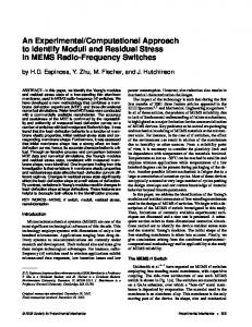
correct but it is useful to m a k e m o r e rigorous tests on their adequacy. Firstly, they have been obtained under the assumption that A ~ 1 which is not necessarily correct. In Fig. 2A we reproduce the distribution of the value of A at each pixel over the entire image. Fig. 2B reproduces similar results obtained for 9 subregions of the image. It is evident that, uniformly over the entire image, for a b o u t 70% of pixels the value of A is less than 0.1. The analysis of the data shown in Fig. 2 indicates that (6), a l t h o u g h not rigorously true, is a reasonable assumption. A further test of the a d e q u a c y of the p r o p o s e d algorithm is the c o m p a r i s o n of the estimated time-to-crash r - that is, the time which elapses before collision with the image plane - with the time-to-crash which can be measured by direct means. The degree of smoothness of the optical flow obtained by means of T R 2 (see Fig. 1D) is very high and adequate for the detection and the local analysis of the focus of expansion PT of the flow. The focus of expansion PT has been located as the point where flow trajectories stop. It can be shown that, if a singular point P is a focus, then z is the ratio between the length of each vector and the distance of the application point of the vector from P (Verri et al. 1988) or more precisely z = 1/;t,
(14)
where 2 is the eigenvalue of multiplicity 2 of the matrix M evaluated at PT. In the optical flow of Fig. 1D, z has been estimated over a n e i g h b o r h o o d containing a h u n d r e d (10 x 10) flow vectors. Indeed, it was found to be nearly constant (mean s t a n d a r d deviation 2.8) and equal to 28.9 time steps, which is in a very g o o d agreement with the true value of 31,1 unit time measured by direct means. The reason for the use of
Fig. 1. A Four frames (256 x 256 pixels) of a sequence of a printed board which translates toward the camera (from the upper lefthand side to the lower right-hand side). The camera is a PULNIX TM46 and the acquisition system consists of the Imaging Technology board FG100. B The optical flow of the third frame of the sequence of A. The optical flow is computed by means of the method described in Sect. 3 with the following parameters: standard deviation of the gaussian used as spatial filter = 5 pixels; standard deviation of the gaussian used as temporal filter= 1 time unit; threshold (maximum speed along each coordinate axis) = 20 pixel/frame. C The same optical flow of B which has been regularized using a subsampling procedure (TRt). The image plane is first divided into non-overlapping squares of n • n pixels. In each square, n estimates of the optical flow for which (12) is best satisfied are selected. Finally, to ensure stability on the data, the estimate corresponding to the smallest conditioning number associated with the linear system of (6) (Bertero et al. 1988) is chosen as representative of the motion field for the whole square. In C a value for n equal to 8 was used. D The same optical flow of B processed according to TR2. The gaussian filter used in the convolution required by TR2 has standard deviation = 8 pixels
83
0.5
m
O
Z
.
0.0
0.2
0.4
0.6
I
I
0.8
1.0
.
.
A
.
.
.
.
.
.
.
.
.
.
.
.
.
.
.
.
.
.
.
.
.
.
.
.
.
.
.
.
,
.
.
.
.
.
.
.
.
9
.
.
.
.
.
.
.
.
.
~
.
9
9
9
~
IIM'rVEIl IIVE,I1
L BL0
.
0
_
.
r
.
.
.
.
.
.
.
.
.
.
.
.
.
.
.
.
.
.
t
.
.
.
.
.
,.
_
,
.
-
9
.
_ 9
.
.
.
.
.
.
.
.
.
.
.
.
.
.
.
"
9
.
"
-
*
9
,
,
,
.
,
9
~
9
.
*
9
9
9
.
.
.
.
.
.
.
.
.
.
.
.
.
-
/
,,
7 0
/
/
/
- . . , . . . . . . . .
10
lo
I
B
~LM~'VEII
/
11~TE'[t
~ C
Fig. 2 A and B. Percentage of pixels on the image plane where (6) is
approximately correct. The correctness of (6) is measured by A= IIMTVEll/IIIZE, II. At the locations where A = 0 , (6) holds exactly. A Distribution of number of pixels at which m- 0.05 < A < ( m + 1). 0.05, m = 0 , ..., 19 over the whole image plane. All the pixels at which A > 1 have been grouped as if 0.95