Mar 26, 2014 - Peppytide workflow and UI mockup-design in Cyborg . . . . . . 73. 4.4 ..... We have designed a web API (Application Programming. Interface) ...
A Computational Framework for Interacting with Physical Molecular Models of the Polypeptide Chain
Promita Chakraborty
Dissertation submitted to the Faculty of the Virginia Polytechnic Institute and State University in partial fulfillment of the requirements for the degree of
Doctor of Philosophy in Computer Science and Applications
Ronald N. Zuckermann, Co-chair Alexey Onufriev, Co-chair Joseph DeRisi Naren Ramakrishnan Liqing Zhang
March 26, 2014 Blacksburg, Virginia, USA
Keywords: Physical models, polypeptides, Ramachandran plot, 3D-printing, molecular model, protein folding, structural biology, biochemistry education, physical-digital interface, macromolecule, Peppytide. ©Copyright 2014 Promita Chakraborty
A Computational Framework for Interacting with Physical Molecular Models of the Polypeptide Chain
Promita Chakraborty
ABSTRACT
Although nonflexible, scaled molecular models like Pauling-Corey’s and its descendants have made significant contributions in structural biology research and pedagogy, recent technical advances in 3D printing and electronics make it possible to go one step further in designing physical models of biomacromolecules: to make them conformationally dynamic. We report the design, construction, and validation of a flexible, scaled, physical model of the polypeptide chain, which accurately reproduces the bond rotational degrees-of-freedom in the peptide backbone. The coarse-grained backbone model consists of repeating amide and α−carbon units, connected by mechanical bonds (corresponding to φ and ψ angles) that include realistic barriers to rotation that closely approximate those found at the molecular scale. Longer-range hydrogen-bonding interactions are also incorporated, allowing the chain to easily fold into stable secondary structures. This physical model can serve as the basis for linking tangible bio-macromolecular models directly to the vast array of existing computational tools to provide an enhanced and interactive human-computer interface. We have explored the boundaries of this direction at the interface of computational tools and physical models of biological macromolecules at the nano-scale. Using a CAD-biocomputational framework, we have provided a methodology
to design and build physical protein models focusing on shape and dynamics. We have also developed a workflow and an interface implemented for such bio-modeling tools. This physical-digital interface paradigm, at the intersection of native state proteins (P), computational models (C) and physical models (P), provides new opportunities for building an interactive computational modeling tool for protein folding and drug design. Furthermore, this model is easily constructed with readily obtainable parts and promises to be a tremendous educational aid to the intuitive understanding of chain folding as the basis for macromolecular structure.
iii
Acknowledgements
First and foremost, I would like to thank my primary advisor Ronald N. Zuckermann at The Molecular Foundry at Lawrence Berkeley National Laboratory. I express my deepest appreciation for having the opportunity to work with him. He believed in me, took risks with a new project, supported me, and provided a very positive and friendly atmosphere towards making the project a success together. This dissertation would not have been possible without his continual support, encouragement, and mentoring. I would like to thank my advisor Alexey Onufriev at Virginia Tech, Department of Computer Science, for his encouragement, support, and advice to keep me on track. I would also like to mention my great appreciation for his professional guidance throughout my dissertation work. I truly cherish the opportunity to have had him as one of my advisors. I am heartily thankful to committee members, Joseph DeRisi (University of California, San Francisco), Naren Ramakrishnan, and Liqing Zhang. I benefited a lot from their scholarly comments, instructions, and guidance. I would like to thank Joseph DeRisi again for graciously letting us use the 3D-printers in his lab at the beginning of the project for our early prototypes. He provided iv
thoughtful follow up comments, encouraging remarks, and he was a part of the first Peppytide video. Thanks to the Bio/Nano/Programmable Matter Group at Autodesk Research, for their support and collaboration. I specially thank Carlos Olguin for the opportunity to work together. I owe my deepest gratitude to Barbara Ryder, the head of the department, Naren Ramakrishnan, Mauel Quinonez-Perez, and Cal Ribbens for their constant help and academic advice throughout my graduate study. I could not have reached this far without their help. I would also like to thank professors in the Department of Computer Science at Virginia Tech, Chris North, Francis Quek, Wu Feng, Clifford Shaffer, Deborah Tatar, and Steve Harrison for their encouragement and support. I thank Molecular Graphics and Computation Facility (supported by National Science Foundation Grant CHE-0840505) at the University of California, Berkeley, for use of the facilities in energy plot computations. I thank my friends and colleagues at Virginia Tech with whom I have spent scholarly as well as leisurely hours. Thank you Anamary Leal, Stacy Branham, Tejinder Judge, Dan Tilden, Joon Suk-Lee, Haeyong Chung, Sirong Lin, Zalia Shams, Bobby Beaton, Michael Stewart, Eric Ragan, Alex Endert, Meg Kurdziolek and Laurian Vega. I will remember all my friends at Virginia Tech’s Association for Women in Computing and all the leadership efforts we made together. Thanks to my friends, colleagues and ex-colleagues at The Molecular Foundry at
v
Lawrence Berkeley National Laboratory, with whom I have spent the last 3 years. Thanks to Rita Garcia and Michael Connolly for their constant help within the lab. Thanks to Gloria Olivier, Caroline Proulx, Babak Sanii, Behzad Rad, Jing Sun, Ranjan Mannige, Thomas Haxton, Helen Tran, and Biljana Mojsoska for proof-reading my papers and providing us useful reference materials. I would also like to thank Anouck Champsaur, Joo(Vicky) Jun, Andrew Cho, and Marika Harada. Thanks to Alison Hatt and Branden Brough at The Molecular Foundry, for their help in the outreach efforts made with Peppytides. Thanks to Frank Kusiak and Rashmi Nanjundaswamy for their helpful advice on collaborating with Lawrence Hall of Science museum. Thanks to Lawrence Hall of Science museum for letting us exhibit our work to visitors. Thanks to Maia Werner-Avidon and Lisa Newton for collaborating with us in user-study evaluation of Peppytide as a learning tool in biology. I thank my friend Urban Wiggins with whom I have had so many positive discussions about work and life. Above all, thanks to my husband, Mehmet Balman, for his constant support. Thanks to my parents Krishna and Tapan, and my sister, Sujata, for their lifelong support in all my endeavors. This work was performed at the Molecular Foundry, Lawrence Berkeley National Laboratory, and was partially supported by the Office of Science, Office of Basic Energy Sciences, Scientific User Facilities Division, of the Department of Energy under Contract DE-AC02-05CH11231. Thanks also to the Defense Threat Reduction Agency and Autodesk, Inc. for funding.
vi
Dedication
To, Everyone who will smile knowingly with the following lines · · ·
To lift a lidyou can say that I am walking with my thumping heart in hand gawking, and eyes blindfolded black, ears in strain; attentively feeling the undulating terrain
with the nerve-endings under my feet, lightly tasting the domain as I tread on yet untouched outstrip overlooking the fact that if I trip, there are things that I would losealong with the blood that would ooze, my heart, then my fingers five five, and eventually my life.
vii
Contents 1 Physical Models in Biology and a Computational Space
1
1.1
Why physical model? . . . . . . . . . . . . . . . . . . . . . . . . . . . . . . .
1
1.2
Motivation for a physical model of polypeptides . . . . . . . . . . . . . . . .
2
1.3
Entity-Relationship between protein and its models . . . . . . . . . . . . . . . . . . . . . . . . . . . . . . . . . . . . .
5
1.4
Thesis synopsis and contribution . . . . . . . . . . . . . . . . . . . . . . . .
7
1.5
Thesis Statement . . . . . . . . . . . . . . . . . . . . . . . . . . . . . . . . .
16
1.6
A brief description of the chapters . . . . . . . . . . . . . . . . . . . . . . . .
16
1.7
Overarching vision . . . . . . . . . . . . . . . . . . . . . . . . . . . . . . . .
17
2 A Coarse-grained Physical Model of Polypeptide Chain
18
2.1
What is a polypeptide? . . . . . . . . . . . . . . . . . . . . . . . . . . . . . .
19
2.2
Design rationale of the physical model . . . . . . . . . . . . . . . . . . . . .
21
2.2.1
The coarse-grained parts . . . . . . . . . . . . . . . . . . . . . . . . .
21
2.2.2
The replaceable side chains
. . . . . . . . . . . . . . . . . . . . . . .
22
Extracting design features from natural polypeptides . . . . . . . . . . . . .
23
2.3.1
Design paradigm: Long-range and short-range interactions . . . . . .
23
2.3.2
Types of short-range interactions in backbone . . . . . . . . . . . . .
23
2.3.3
Quantifying rotational barriers in backbone dihedral angles . . . . . .
28
2.3
viii
2.3.4
Representing the biases in φ and ψ . . . . . . . . . . . . . . . . . . .
31
2.3.5
Long-range interactions . . . . . . . . . . . . . . . . . . . . . . . . . .
34
2.4
Model assembly . . . . . . . . . . . . . . . . . . . . . . . . . . . . . . . . . .
34
2.5
Alanine di-peptide: The smallest peptide . . . . . . . . . . . . . . . . . . . .
42
2.6
Scale of model . . . . . . . . . . . . . . . . . . . . . . . . . . . . . . . . . . .
43
2.7
3D printing an entire model . . . . . . . . . . . . . . . . . . . . . . . . . . .
44
2.8
Designing for specific proteins . . . . . . . . . . . . . . . . . . . . . . . . . .
45
2.9
Summary . . . . . . . . . . . . . . . . . . . . . . . . . . . . . . . . . . . . .
46
3 Folding with Physical Models 3.1
47
Folding in Peppytides . . . . . . . . . . . . . . . . . . . . . . . . . . . . . . .
47
3.1.1
Why physical models to study folding? . . . . . . . . . . . . . . . . .
47
3.1.2
Which folded structures we explored and why? . . . . . . . . . . . . .
48
3.1.3
Folding and measurement of α−helix . . . . . . . . . . . . . . . . . .
49
3.1.4
Folding and measurement of β−sheets . . . . . . . . . . . . . . . . .
52
3.1.5
Folding of β−turns . . . . . . . . . . . . . . . . . . . . . . . . . . . .
54
3.1.6
A comparison between 310 helix, α−helix and π−helix . . . . . . . .
57
3.2
Tertiary structures . . . . . . . . . . . . . . . . . . . . . . . . . . . . . . . .
57
3.3
Discussion . . . . . . . . . . . . . . . . . . . . . . . . . . . . . . . . . . . . .
59
3.3.1
Backbone flexibility . . . . . . . . . . . . . . . . . . . . . . . . . . . .
60
3.3.2
Unfolding of the α−helix to β−sheet in Peppytides . . . . . . . . . .
61
3.4
Advantages of folding a customized model over generic model
. . . . . . . .
63
3.5
Summary . . . . . . . . . . . . . . . . . . . . . . . . . . . . . . . . . . . . .
64
4 Towards a Computing Paradigm for Physical Biomodels 4.1
A brief history of the physical-digital space . . . . . . . . . . . . . . . . . . . ix
65 66
4.2
The concept of a physical-digital paradigm for biology . . . . . . . . . . . . .
4.3
A methodology for the physical-digital paradigm for polypeptides at nano-scale 70 4.3.1
69
Biomodeling platform for Peppytide digital representation: The Peppytide API . . . . . . . . . . . . . . . . . . . . . . . . . . . . . . . . . . . .
71
4.3.2
Digital representation: Simulating the physical model . . . . . . . . .
74
4.3.3
The workflow for digital-physical interfacing of Peppytides . . . . . .
75
4.3.4
The Cyborg and Nucleus Autodesk platforms . . . . . . . . . . . . .
77
4.4
Parameterizing to enable design of specific proteins . . . . . . . . . . . . . .
77
4.5
A grammar for model checking of backbone . . . . . . . . . . . . . . . . . .
83
4.6
Capturing physical model with camera: From physical model to digital form
85
4.7
Augmented reality and virtual reality in biology . . . . . . . . . . . . . . . .
86
4.8
Framework for data flow in physical-digital platform . . . . . . . . . . . . . .
88
4.9
Summary . . . . . . . . . . . . . . . . . . . . . . . . . . . . . . . . . . . . .
90
5 Application and Impact in Society
91
5.1
Use in informal learning environment . . . . . . . . . . . . . . . . . . . . . .
92
5.2
Use in classroom . . . . . . . . . . . . . . . . . . . . . . . . . . . . . . . . .
98
5.3
Summary . . . . . . . . . . . . . . . . . . . . . . . . . . . . . . . . . . . . .
98
6 A New Direction in Biomodeling and Future Possibilities
99
6.1
A viable input device for molecular chains . . . . . . . . . . . . . . . . . . . 100
6.2
A viable output device for molecular chains? . . . . . . . . . . . . . . . . . . 101
6.3
Possibilities for self-folding and biomimetic modular robotics . . . . . . . . . 101
6.4
Other possibilities . . . . . . . . . . . . . . . . . . . . . . . . . . . . . . . . . 103
6.5
Study of misfolded proteins and aggregates . . . . . . . . . . . . . . . . . . . 103
6.6
Electrostatic and hydrophobic interactions . . . . . . . . . . . . . . . . . . . 104 x
6.7
Exploring other types of polymers . . . . . . . . . . . . . . . . . . . . . . . . 104
7 Conclusion
106
Bibliography
109
Appendices
123
A STL files for 3D printing
124
B Model specifications
126
C Drilling dimensions
130
D Determination of the rotational energy barrier profile for the circular magnet array
132
E Supporting movies
136
E.1 About Peppytides . . . . . . . . . . . . . . . . . . . . . . . . . . . . . . . . . 136 E.2 Folding Peppytides . . . . . . . . . . . . . . . . . . . . . . . . . . . . . . . . 138 F A few useful website resources
140
F.1 A server for β−turn types prediction . . . . . . . . . . . . . . . . . . . . . . 140 F.2 Scripps Physical Model Service . . . . . . . . . . . . . . . . . . . . . . . . . 144 F.3 Center for Biomolecular Modeling, Milwaukee School of Engineering . . . . . 147
xi
List of Figures 1.1
The Entity Relationship between real-world proteins, computational models and physical models. . . . . . . . . . . . . . . . . . . . .
1.2
Exploring relationship between existing computational models and experimental data from native protein structures.
1.3
. . . . .
9
Exploring relationship between experimental data from native protein structures and physical model of polypeptides. . . . . .
1.4
6
11
Exploring relationship between existing computational models, other emerging computing paradigms and physical model of polypeptides. 13
1.5
An unexplored computational space. . . . . . . . . . . . . . . .
15
2.1
Exploring Process 3: From natural proteins to physical models .
19
2.2
Representations of the repeating units of the polypeptide chain
20
2.3
A comparison of the side chain models for the amino acids. . . .
23
2.4
Shapes and dimensions of the repeating units in the polypeptide chain model . . . . . . . . . . . . . . . . . . . . . . . . . . . . .
2.5
24
Distribution of φ and ψ bond angles in the polypeptide chain, and in the Peppytide model . . . . . . . . . . . . . . . . . . . .
26
2.6
Van der Waals radius of atoms in benzene . . . . . . . . . . . .
27
2.7
Enforcing rotational barriers on the φ and ψ bonds using circular magnet arrays . . . . . . . . . . . . . . . . . . . . . . . . . . . . xii
30
2.8
Peppytide model assembly . . . . . . . . . . . . . . . . . . . . .
33
2.9
Steps of assembly: Amide unit. . . . . . . . . . . . . . . . . . .
36
2.10
Steps of assembly: Alpha carbon unit. . . . . . . . . . . . . . .
37
2.11
Steps of assembly: Assembled bonds and related parts that need to be linked per repeating monomer unit. . . . . . . . . . . . .
38
2.12
Steps of assembly: Alpha carbon unit with bond linkages. . . .
39
2.13
Steps of assembly: Connecting the alpha carbon unit with the two faces of amide units. . . . . . . . . . . . . . . . . . . . . . .
40
2.14
Assembling backbone . . . . . . . . . . . . . . . . . . . . . . . .
41
2.15
Final assembly of side chains . . . . . . . . . . . . . . . . . . .
41
2.16
Helix Template . . . . . . . . . . . . . . . . . . . . . . . . . . .
42
2.17
Alanine di-peptide . . . . . . . . . . . . . . . . . . . . . . . . .
43
3.1
Exploring Process 4: From physical models to natural proteins .
48
3.2
Peppytide folded into α−helix, a secondary structure. Comparison of a 13-mer polyalanine α−helix (RM = 0.7RV DW ) . . . . . . .
3.3
Peppytide folded into β−sheets. Two strands of polyalanine Peppytide model folded into β−sheet conformations. . . . . . .
3.4
51
53
Folded β−turn secondary structures, types I and II, formed with the Peppytide model. . . . . . . . . . . . . . . . . . . . . . . . .
54
3.5
Type I, I� , II, II� β−turns made with Peppytide . . . . . . . . .
56
3.6
A comparison between 310 helix, α−helix and π−helix . . . . .
57
3.7
Protein structural motif with Peppytide . . . . . . . . . . . . .
58
3.8
Tertiary structure of Fish Osteocalcin . . . . . . . . . . . . . .
59
xiii
3.9
Transition of α−helix to β−sheet in Peppytide due to an applied torsional unraveling force on both sides. . . . . . . . . . . . . .
4.1
62
Exploring Process 5: From computational models and CAD to physical models . . . . . . . . . . . . . . . . . . . . . . . . . . .
67
4.2
Physical model and digital platform
. . . . . . . . . . . . . . .
70
4.3
Peppytide workflow and UI mockup-design in Cyborg . . . . . .
73
4.4
The design of workflow for implementing physical-digital Peppytides through the Cyborg platform. . . . . . . . . . . . . . . . . . . .
4.5
75
Rotational barrier for generic polypeptide backbone. (a) phi-face, (b) psi-face. . . . . . . . . . . . . . . . . . . . . . . . . . . . . .
78
4.6
The parameters for the main workflow and the digital representation 81
4.7
The parameters for the digital-physical representation
. . . . .
82
4.8
A graphical representation of backbone grammar . . . . . . . .
85
4.9
Exploring Process 6: From physical models to computational models . . . . . . . . . . . . . . . . . . . . . . . . . . . . . . . .
86
4.10
Physical model as input device. . . . . . . . . . . . . . . . . . .
87
4.11
Framework of data flow between physical and computational models. . . . . . . . . . . . . . . . . . . . . . . . . . . . . . . .
5.1
89
Protein structures shown to users: Trichosurin, a milk-whey protein; Dendrotoxin K, snake venom from black mamba; Keratin, found in hair (and skin). . . . . . . . . . . . . . . . . . . . . . .
93
5.2
Visitor interest in various activities . . . . . . . . . . . . . . . .
95
5.3
Visitor interest in exhibit item and physical models of polypeptides 96
5.4
Visitor response when asked “What did you build?” . . . . . . . xiv
97
C.1
Detailed drilling and assembly plan of Peppytide. . . . . . . . . 131
D.1
A simple torqometer was used to monitor current drawn by the rotational barrier magnet arrays as a function of bond angle. . . 133
D.2
Data processing steps in converting the torqometer current data into the rotational barrier data. . . . . . . . . . . . . . . . . . . 135
E.1
Peppytide video screenshots . . . . . . . . . . . . . . . . . . . . 137
E.2
Folding with Peppytides (video screenshots) . . . . . . . . . . . 139
xv
Chapter 1 Physical Models in Biology and a Computational Space
1.1
Why physical model? Shapes are ubiquitous in nature. Yet, computational science and engineering
struggle to represent and manipulate algorithms related to shapes (computational geometry), and to extract shapes (computer vision) from the 3-dimensional world. The dynamics of these structures further add to the complexity. Biological structures, from the nano-scale to macro-scale are known to flex, fold, grow or shrink, and are constantly evolving from one form to another. A remarkable example of complex dynamic structures is the protein folding problem. Simulations provide a successful means to study the phenomenon, but they still lack a platform that will facilitate an intuitive understanding of the underlying complexity.
1
On the other hand, form-specific physical objects are easy to manipulate by hand, and can be designed to emulate the shape and mechanics of bio-systems. The interplay between the physical and computational models can be analyzed, evaluated and designed to contribute in a complementary manner, so that the two can work together to provide a more effective tool. A new paradigm emerges from this analysis wherefrom the form and flexibility of the real-world object can contribute to the better parameterization of the computer models, and to a deeper intuition of the biological phenomena.
1.2
Motivation for a physical model of polypeptides Understanding protein folding pathways, predicting protein structure and the
de novo designing of functional proteins have been a long-standing grand challenge in computational and structural biology. Although tremendous advances are being made [2], folded protein structures are very difficult to visualize in our mind due to their complexity and shear size. State-of-the-art computer visualization techniques are well developed and provide an array of powerful interactive tools for exploring the 3D structures of biomacromolecules [3– 5]. While increasingly complex molecules can be visualized with computers, the mode of user interaction has been mostly limited to the mouse and keyboard. Although the use of haptic devices is on the rise, there are only a few low-cost, specialized input devices particularly designed for interaction with biomacromolecules. Augmented-reality (AR) and immersive environments enhance user interaction experiences during the handling of existing Remarks in this section are based on our contribution on physical model of polypeptides in our paper titled“Coarse-grained, foldable, physical model of the polypeptide chain” published in PNAS, 110(33), (2013) [1]. 2
visualization tools [3,6,7], but the physical models used in these environments are not flexible or precise enough to represent the conformational dynamism of polypeptides by themselves. There is a strong need for scaled, realistically foldable, but inexpensive, physical models to go hand-in-hand with the AR and other computer interfaces, while concomitantly taking better advantage of current computational capabilities. Physical molecular models of organic small molecules and biomacromolecules with atomic representations have been around for many decades [8–18]. Although early pioneers like Pauling and Corey’s scaled physical model of the polypeptide chain [12] helped to elucidate the molecular packing details of protein secondary structures [16, 18], these were non-flexible models and did not capture the inherent dynamism now known to exist in protein structures. Although there are a variety of physical molecular models commercially available [10, 11, 14, 15, 17], none have captured the true conformational degrees of freedom of the polymer chain, as the macromolecules have too many atoms, complex short-range and long-range conformational constraints, and specific folding behaviors. There are construction kits for α-helices, β-sheets, and nucleic acids [15] that capture the scale and complexity of these molecules, but they are not flexible. Some models focus on chemical structures with multiple types of bonding [10] but are not made to scale. Other models spontaneously self-assemble into 3D molecules aided by internal magnetic fasteners [17] but are too simplistic to represent the folding of the polypeptide chain. Entire molecules of folded protein structures have also been generated with 3D printing, but these models do not explicitly represent the back- bone and thus cannot be folded or unfolded. Although many of the existing models are accurate with respect to physical dimensions (atomic radii, bond lengths, and bond angles), none is able to freely sample the
3
bond rotational degrees of freedom that are needed to represent the motion of the polypeptide chain. The most dynamic representation reported is Olson’s articulated model that has been used to make flexible polypeptides by chaining the constituents through an elastic string, with the elasticity representing the pull between atoms [19]. These models are flexible and can be folded into protein secondary and tertiary structures, but do not have the space-filling impact or a realistic representation of the dihedral angle rotational barrier that are so central to protein backbone behavior. Despite these limitations, physical models have been rising in popularity [8, 9], as they play a critical role, both as educational tools and as aids to chemistry and biochemistry researchers to gain insight into protein-folding mechanisms. Physical models engage visuospatial thinking of biomolecules much more effectively than textbook images and computer screens can, via a process termed “tactile visualization” [20]. Moreover, experiments with gaming interfaces like FoldIt have demonstrated that humans have superior 3D pattern matching skills than any existing software for solving challenging scientific problems [21, 22]. We believe that this intuition and skill can be even more channelized while playing with physical, foldable models and may result in unexpected and surprising discoveries, as in the case of FoldIt. With this vision in mind, we designed and fabricated a tangible, coarse-grained, dimensionally accurate, physical molecular model of the polypeptide chain, which has the necessary degrees of freedom and bond rotational barriers to accurately emulate the backbone folding dynamics of the polypeptide chain [1]. Our approach was to break down the component amino acids into constituent coarse-grained components linked by rotatable bonds. The flexibility of the backbone chain in our model has made it possible to readily build all of the
4
common protein secondary structure elements. This model, named Peppytide, is a necessary first step toward a sophisticated computer input device that can manipulate and intuitively interact with computer visualization tools. It should ultimately be possible for these models to provide interactive dihedral angle information to computers while transitioning between various conformations. This would enable real-time feedback about the chain’s conformational energy and direct comparison with known protein structures (structural homology searching). The model will serve as a first step in implementing an intuitive, computationally augmented physical model that can help people instinctively understand and hypothesize new details about the science of protein-folding pathways.
1.3
Entity-Relationship between protein and its models We have been able to establish the mapping between Peppytides (the physical
model that we designed) and natural proteins. All possible folding of natural proteins can be achieved with Peppytides, and conversely, a structure made with Peppytides is a possible candidate for a protein(s) or its subpart(s). A mapping of the physical model to its digital counterpart makes possible a two-way interaction between Peppytide and the existing biomodeling tools like PyMOL [23],VMD [24], and Chimera [25]. Supporting Movie in Appendix E provides an introduction to the features of Peppytide. With the two types of modeling approaches available to us, with computational and physical models, we analyze the relationship-triangle that exists between the natural
5
proteins, the computational models for protein folding, and the physical model of the polypeptide chain (Figures 1.1 and 1.3). Section 1.4 describes in detail how these are related.
(b) The processes we explored: Physical objects,
(a) Control flow for protein folding models and
computational models and native state protein
experimental data.
structure data are all intertwined.
Figure 1.1: The Entity Relationship between real-world proteins, computational models and physical models.
6
1.4
Thesis synopsis and contribution Over the last 50 years, bioinformatics and computational biology has revolutionized
the way we do research in biology. Since the mid-twentieth century, increasing amount of data from experiments, biological sequencing, structure determination and phylogenetic studies have eventually fueled and outlined the developments in these two disciplines. Addressing these problems have in turn fed forward to developments in various branches within computer science including algorithms, graph theory, computational modeling, parallel computation methods, pattern recognition and visualization. The prevalence of visualizing tools repeatedly highlights the eternal human need for spatial understanding, to orient their insights in terms of geometry. However, the current biocomputational approaches leave tangibility and geometry at the periphery. With the recent developments in 3D-printing and CAD technologies it will now be possible to explore the convergence of these domains within biocomputation. The biocomputational models till date that focus on structure and dynamics of macromolecules, have limited themselves to modeling in terms of force fields, energy and entropy. The dynamics is thought of as entropy minimization problem. Even though these are precise methodologies for studying shapes and dynamics in the protein folding process, the embodiment of properties within physical models – the tangibility-factor – is still hard to capture given the complexity of biological systems. There is a void, a need felt for direct representation and manipulation of these shapes that can have both physical and digital presence. In recent years, extensive studies have been made in CAD methodologies, solid
7
modeling geometry and 3D printing techniques. But biology research community is yet to gain from these advancements. A marriage of 3D CAD and biocomputation is in sight with cutting-edge technologies like 3D bioprinting of tissues [26,27], DNA origami with CAD-Nano and DNA scaffolds [28,29]. These are transformative and disruptive technologies from which the society will greatly benefit in future. The questions that come to mind is: What happens if we want to build macro-scale, precise physical models of any of these? Can these models actually serve as instruments for future studies – and if this is indeed possible, can we imbibe digital knowledge into them so that they can “compute” by virtue of the shape and dynamics? We define 3 sets as: N (Natural proteins):
Data
from
native
protein
structures,
experimental analysis and observations C (Computational models):
Existing computational models and the data generated from them
P (Physical models):
Form-specific physical models of proteins
We explore the relationship between these sets to identify their current scopes and to pinpoint the unexplored areas that will complement the existing computing frameworks.
8
Figure 1.2: Exploring relationship between existing computational models and experimental data from native protein structures.
Numerous studies have been done in attaining precise computational models and folding principles using template matching, force field calculations and other methods [2, 30, 31], as it is an extremely important topic that has implications for medicine and drug design in addition to understanding the fundamental rules of protein folding (Process 1). Studies have also been made in designing small de novo proteins with less that 40% homology to known sequences to achieve a preferred structure [32, 33] (Process 2). This body of work have firmly established the relationship between the protein folding data available from X-ray crystallography and NMR structures of native states, and the de novo protein folds (Figure 1.2). Though there have been tremendous advances in computational techniques for 9
protein folding, the building of flexible physical models or tying them to computational resources, have remained completely unexplored. We have explored the boundaries of a new direction of research at the interface of computer science and the nano-scale biological macromolecules by tying together the concepts of form-specific physical-digital interfaces. We see a new computational space at the intersection of the sets N , C and P . With these observations, a new computational paradigm emerges for physical-digital interfaces for studying of protein folding that focuses on shape and dynamics. For prototyping and proof-of-concept of the principle, we have developed a scaled physical model of the polypeptide chain, called Peppytides, and established its accuracy and ability to form various folded secondary and tertiary structure motifs found in proteins at their native states [1] (Process 3, Figure 1.3, details in Chapter 2). We then tested the model by folding it manually into a variety of secondary structures (Chapter 3). The right-handed helices that we made are the ubiquitous α−helix, and the less frequent 310 helix and π−helix found in proteins. Left-handed helices are not so common in nature. We made the parallel and anti-parallel β−sheets, the two types of possible β−sheets. We made the beta−turn types frequently found in nature. For tertiary structure, we made the ββα motif, one of the most common motifs found in proteins, and a small protein, Osteocalcin, found in bones of animals. Thus, with these folds in Peppytides we have established a bijective mapping between the physical model and the native structures of proteins. This implies that the structures we can make with the model is possible in proteins and vice versa (Processes 3 & 4, Figure 1.3).
10
11
Figure 1.3: Exploring relationship between experimental data from native protein structures and physical model of polypeptides.
We further represented the model digitally and have worked towards binding it to computational platforms. We have designed a web API (Application Programming Interface) platform where users can design their own physical model of the polypeptide, and then 3D-print the parts for final assembly (Process 5, Figure 1.4, Section 4.3). This is possible because of the digital representation serving as the underlying knowledge base at its core. This mapping enables an easy conversion of the design principles of CAD-oriented modeling to biological macromolecules (polypeptides) and vice versa. This prototype is a proof-of-concept that marrying CAD-based platforms, 3D-printing and physical models with biocomputational simulations, opens up new possibilities for research in biology with macro-scale models. With such a platform, we hope to be able to digitally fold, unfold, and assemble the physical-digital model using self-assembly simulations, and also verify the folds in hand with the physical model. Such features will serve useful purposes for users who would like to: (a) 3D-print, assemble and fold a physical polypeptide model, and (2) simulate the behavior of the physical model, so as to take into considerations its physical parameter constraints like weight and magnet strengths. Thus, we see a void and a need for biomodeling platforms and modeling languages that will not only deal with CAD and macro-scale physical design environment, but will also have a way to port to the latest biomodeling tools in future, like ROSETTA for protein folding computations [31, 34]. We need a framework and the guiding principles that will glue these two platforms together, paving the way for new standards for these novel file formats.
12
13
Figure 1.4: Exploring relationship between existing computational models, other emerging computing paradigms and physical model of polypeptides.
A natural next-step would be to capture the structure of the physical models which could then be represented digitally in real-time (Process 6). Similar kinds of object tracking experiments have been made with lego blocks where a Microsoft Kinect camera, with depth-sensing feature, tracks the building up of an object from constituent lego parts [46,47]. Through exploration of Processes 1-6, we see that a relationship-triangle exists between the natural proteins (P), the computational models for protein folding (C), and the physical models of the polypeptide chain (P) with bijective mapping between the sets (Figure 1.5). We arrive at a computational space at the intersection of N, C and P that has so far remained unexplored, possibly because of the difficulty in designing and fabricating accurate, scaled physical models of polypeptide chains along with its complex degrees-of-freedom. Now with 3D-printing technologies, and possibilities for CAD-cum-biocomputation platforms, we are poised to explore this new domain.
14
15
Figure 1.5: An unexplored computational space. (a) The Entity-Relationship diagram in the physical-digital computing model, (b) The unexplored computational space at the intersection of N, C and P, (c) Scenarios and applications that belong to this computational space.
We see the emergence of a new paradigm resulting from this analysis. The computational space uncovered sets forth new ways to think about bio-macromolecules that complement the existing methods. This paradigm may be further extended to include other topics in biology, using similar principles.
1.5
Thesis Statement In this dissertation we explore the boundaries of a new direction of research at the interface of computer science and biological macromolecules at the nano-scale. We uncovered a previously-unexplored computational space. We tie together the concepts of form-specific physical-digital interfaces, CAD modeling and biocomputational platforms. With these principles, a new computational paradigm emerges for studying biological systems that focus on shape and dynamics.
1.6
A brief description of the chapters In Chapters 2 and 3, we discuss the design of a scaled physical model of polypeptides.
We extend our work titled“Coarse-grained, foldable, physical model of the polypeptide chain” published in PNAS, 110(33), (2013) [1] and introduce our model, Peppytide, in which we emulate basic structure of the polypeptide chain backbone. We establish the model’s accuracy and ability to form various folded structures found in proteins at their native states. Herefrom, it opens the door for a bijective mapping between the physical model and 16
its digital representation, towards the goal of a computer-interfaced, intuitive platform for biomodeling, which we discuss in Chapter 4. This work provides opportunities for usage of this framework for teaching and future research possibilities. In Chapters 5, we outline some of the applications we have already explored for learning and teaching. As these concepts open up a new direction in biomodeling tools, in Chapter 6, we outline the possibilities for future investigations and the research prospects that lie ahead of us in this new direction with the help of existing and emerging technologies. In Chapter 7, we summarize the essential high-points of the dissertation and provide concluding remarks.
1.7
Overarching vision We envision that this is the first step to scaled physical models of proteins of
the future, which not only will self-assemble and unfold automatically, but will also inform us about the spatio-temporal aspects of folding pathway. Thinking ahead, such models would have great implications scientifically, such as providing intuition and insights to drug designers about how small-molecules bind and how to disrupt protein-protein interactions. We foresee that the interactions between physical and computational models will enable novel approaches for scientific discovery making way for new computing paradigms.
17
Chapter 2 A Coarse-grained Physical Model of Polypeptide Chain
In this chapter we explore the design of a physical model of polypeptides (Process 3, Figure 2.1). We establish that the behaviors of polypeptides can be captured and encapsulated within this physical model through use of parameters like size of atoms, long-range and short-range interactions. As a first step towards building a computer-augmented physical polypeptide model that may have applications in structural biology and drug design, we have designed, fabricated and validated this dimensionally accurate, physical model of the polypeptide chain, that has a flexible backbone where the dihedral bonds are rotationally constrained to match their molecular counterparts. We have reproduced all the backbone degrees-of-freedom to better understand folding dynamics of the chain.
18
Figure 2.1: Exploring Process 3: From natural proteins to physical models
2.1
What is a polypeptide? A polypeptide is a linear sequence of amino acids connected together by peptide
bonds or amides (Figure 2.2a). In natural polypeptide chains or proteins, the bond rotations along the linear backbone are restricted, such that only certain bonds can rotate while others remain relatively rigid. By studying these rigid and rotation behavior of natural polypeptides, we can extract the essential characteristics and consolidate them in a physical model. The atoms which remain rigid to each other can be modeled as a single part so that each distinct part is a coarse-grained unit that together represent a monomer in the physical model with the units rotating with respect to each other. Each amino acid monomer contains two backbone rotational degrees of freedom, the φ and ψ dihedral angles (the red bonds in Figure 2.2b), about which the rigid units 19
rotate. In this chapter, I discuss how these rigid units and the rotating bonds work in unison to represent a coarse-grained molecular model of the polypeptide chain.
Figure 2.2: Representations of the repeating units of the polypeptide chain. (a) A repeating homopolymer of amino acid units connected by amide bonds (red). (b) An alternating copolymer of rigid amide (green) and α−carbon (blue) units connected by the rotatable bonds φ and ψ (red).
20
2.2
Design rationale of the physical model When we consider the rigid and flexible backbone elements, the chain can be
dissected into two repeating units: a set of four atoms confined to a rigid plane (forming the amide), and the α−carbon atom, where two amides are connected via φ and ψ bonds. Thus, the polypeptide backbone can be represented as an alternating copolymer of the amide unit and the α−carbon unit.
2.2.1
The coarse-grained parts In our model, referred to as a Peppytide, we emulate this basic structure of the
polypeptide chain backbone by linking two types of units together: the amide units and the α−carbon units (Cα ), connected alternately at φ and ψ bonds (Figure 2.4 c and d). Figure 2.2b shows the green amide units and the blue α−carbon unit. We first tested a generic polypeptide chain model with a methyl-group unit (Figure 2.4e) representing the hydrophobic amino acid alanine. We chose alanine to be the first representative side chain of the generic model because it is the smallest amino acid side chain where the methyl group can approximate the impact of side-chain substitution and chirality and the general dynamics of a small peptide chain. Poly-alanine, that is, multiple alanines in sequence Ala − Ala − Ala − · · · , has also been known to form α−helices and β−sheets [35, 36]. So it seemed logical to test the accuracy and foldability of the generic physical poly-alanine model by folding it into the secondary structures, as described in Chapter 3.
21
2.2.2
The replaceable side chains Looking closely into the structure of amino acids in polypeptides, the amides
and the α−carbon units alternately forms the backbone of the chain. These are the parts common to all the amino acids. For unique sequences of amino acids, only the side chain structure changes from one amino acid to another. Thus, we can have the entire array of possible sequences of amino acids represented by these models simply by keeping the backbone as it is while interchanging among the side chain portions. For example, if we want to make a sequence of Alanine − V aline − Glycine using the physical model, all we need to do is to push the side chains for alanine, valine, and glycine in place in this sequential order connected to the α−carbon unit, while keeping the backbone as is. To make a sequence of V aline − Glycine − Alanine just interchange these side chains to get this order, and so on. In a nutshell, in Figure 2.8c the black and white amide and α−carbon units remain connected as is, and we just replace the blue side-chain part for the required side chain part. The simple design of the model makes it ideal for further elaboration. An obvious next step is to expand to the full set of amino acid side chains, so that a complete protein tertiary structure can be folded. We have developed a few set of units for the replaceable side chain residues of the amino acids. Figure 2.3 shows an implementation of Valine’s side chain. Henceforth, we are extending the residues to a full set of amino acid side chains.
22
Figure 2.3: A comparison of the side chain models for the amino acids. Alanine (left) and Valine (right)
2.3 2.3.1
Extracting design features from natural polypeptides Design paradigm: Long-range and short-range interactions Polypeptide backbone conformations are dominated by both short-range interactions
about φ and ψ, and longer-range intra-chain hydrogen bonding interactions, as well as the interactions of the side chains. The Peppytide model embodies both the short-range and long-range interactions of the backbone in addition to the steric hindrances of atoms that are within spatial proximity.
2.3.2
Types of short-range interactions in backbone The factors most important for steric hindrances are the shapes and sizes of the
constituent parts. By close analysis of protein crystal structures, the shapes of amide units (trans) and α−carbon units (corresponding to L-amino acids) were designed (Figure 2.4a).
23
Figure 2.4: Shapes and dimensions of the repeating units in the polypeptide chain model. (a) Equivalence of the shape of amides and α−carbons in a leucine zipper motif (from pid:2ZTA), and that of the Peppytide model; C, green; H, gray; N, blue; O, red. (b) Bond dimensions and angles of atoms drawn to scale, comprising amides and α−carbons used for the model [37]. (c-e) CAD drawings and finished parts: (c) α−carbon unit corresponding to L-amino acids: ψ-face (Upper Left); φ-face (Upper Right); side-chain face (Lower Right), (d) amide unit (trans configuration): φ-face (Upper); ψ-face (Lower). (e) Methyl-group unit (for alanine side chain). The most widely accepted values of interatomic distances have been used for the atomic-scale dimensions of the units (Figure 2.4b) [37]. All parts were drawn to scale with a scale factor of 1˚ A = 0.368�� in a computer-aided design (CAD) software (Figure 2.4 c-e). The φ and ψ bonds, which are the linkages between the amide and α−carbon units, were implemented with freely (360°) rotating nut-and-screw arrangements. Rotational barriers were also included to 24
reproduce the dihedral angle preferences observed in protein structures (see below). As the constituent atoms of each of the units need to be within their covalent bonding distances, the bonding atoms were cut along specific planes, as had been previously done with the Corey-Pauling-Koltun (CPK) and other models [12].
25
Figure 2.5: Distribution of φ and ψ bond angles in the polypeptide chain, and in the Peppytide model. (a and b) Distribution of φ and ψ bond angles from 77,873 protein structures (∼ 59 million points) from the PDB: (a) φ has two peaks (energy minima positions) at −62° and −118°. (b) ψ has two peaks (energy minima) at −42° and 138°. (c) Effects of steric hindrance on the conformational flexibility in the Peppytide model (measured at 5° intervals) for atom radii of 0.6, 0.7, and 0.8 RV DW , respectively (from Left to Right). (d) Ramachandran histogram plot representation of the PDB data from A and B. (e) Ramachandran energy plot from the quantum mechanical OPLS force field calculations computed at 1° intervals using alanine di-peptide molecule in the Maestro platform (in kilocalories per mole). (f) Measured energy landscape of the Peppytide model resulting from the magnet array rotational barriers of φ and ψ bonds. The darkest blue circles are the energy minima dictated by the magnet arrays. The red regions in c and f represent sterically inaccessible conformations due to occlusion between parts. 26
Theoretically, the atom size for the elements in the backbone chain, namely the model radii (RM ), in any model should be equal to their Van der Waals radius (RV DW ). Figure 2.6 shows a study of the relationship between the space-filling effects of atoms and their Van der Waals radiii in benzene. However, in a dynamic physical model, the RM needs to be a fraction of RV DW for the chain to move freely and avoid getting interlocked with itself. This was examined by checking for steric clashes in a CAD software using a 3D drawing of the alanine diamide molecule assembled using Peppytide model units. RM was varied from 0.6 RV DW to 0.8 RV DW (Figure 2.5c), and it was found that RM = 0.7 RV DW is the largest size possible for representing hard spheres while maintaining access to the entire conformational landscape accessible by polypeptides. To get a quick sense of the differences in size between these values, Figure 2.6 shows a comparison of the fractional radius of atoms in benzene.
Figure 2.6: Van der Waals radius of atoms in benzene. 27
2.3.3
Quantifying rotational barriers in backbone dihedral angles The backbone dihedral angles in polypeptide chains do not rotate freely. There
are barriers to rotation about both φ and ψ that limit the conformational flexibility of the chain, which is a result of the local bonding geometry, steric and electronic effects [38]. We therefore introduced a conformational bias into each rotatable bond in the backbone of the model. The favored dihedral angles (φ, ψ) in polypeptides are well known from experimental data and are typically illustrated in a Ramachandran plot [38]. The densest regions of the plot, that is, the most favorable regions, are low-energy positions of dihedrals of the polypeptide backbone (Figure 2.5d). These preferred regions mostly correspond to the α−helix (left- and right-handed) and the β−sheet conformations – the secondary structures universally found in proteins. To represent these barriers within the physical model, it was necessary to decouple φ and ψ from each other and to study their behavior separately. The information from the Ramachandran plot was decoupled to get independent values of φ and ψ over the full range of rotation (180°, 180°) (Figure 2.5 a and b). We used data from approximately 78,000 known protein structures in the Protein Data Bank (PDB) because these data are a direct manifestation of the favored angles adopted in proteins. For comparison, we also generated a Ramachandran energy map with OPLS 95 (optimized potentials for liquid simulations) force fields in the Maestro framework for alanine di-peptide, where the energy minima mostly clusters around φ = −70° and ψ = 140° (Figure 2.5e). However, these calculated energies are an indirect measurement of the same effect as they reflect only very local interactions. As we wanted to incorporate the effects of both short-range and long-range interactions in the physical model, we used the data from the PDB histogram instead of the minima in the 28
energy maps to design the rotational barriers. The decoupled φ and ψ distributions giving preferred angles for φ and ψ (Figure 2.5 a and b) were calculated from ≈ 59 million (φ, ψ) values obtained from 77,873 protein structure files from the PDB (crystallography and NMR structures only). The four peaks obtained (two for φ; two for ψ) correspond to the darkest regions of the Ramachandran plot for α−helix and β−sheet conformations, and denote the corresponding minimum energy configurations. This analysis shows that the φ-peaks are 56° apart (at −62° and −118°) and ψ-peaks are 180° apart (at −42°, 138°). There is a third φ-peak at ∼ 61° that corresponds to left-handed helices, which is not represented in this version of the model. The peaks in the φ and ψ distributions were each fit to Gaussian distribution (Figure 2.5a) to facilitate their approximation in the physical model. To introduce these dihedral angle preferences, or rotational barriers into the physical model, we used a customized circular magnet array for each φ and ψ bond. Magnet arrays can be quite intricate and can produce a wide variety of mechanical interactions [39, 40]. Magnets are attractive choice in this application because they are non-contact, frictionless, cheap, passive (need no power to operate), exhibit strong coupling behavior, and can generate Gaussian barriers.
29
Figure 2.7: Enforcing rotational barriers on the φ and ψ bonds using circular magnet arrays; N, north pole; S, south pole. (a) (Left) The coupled faces for φ, simulating the rotational constraints on φ; peaks are 56° apart. (Center) φ-faces of the amide and α−carbon units. (b) (Left) The coupled faces for ψ, simulating the rotational constraints on ψ; peaks are 180° apart. (Center) ψ-faces of the amide and α−carbon units. (a and b) (Right) The measured energy landscape for φ (Upper) and ψ (Lower) in the model corresponding to magnet arrangements (red), overlaid with the distribution of φ and ψ from protein structures (blue) for performance comparison; (Insets) the coupling of interface magnets that lead to the respective peaks in the model, blue (φ-face), red (ψ-face).
30
2.3.4
Representing the biases in φ and ψ In Peppytides, we reproduced the conformational biasing due to rotational barriers
by two separate arrangements of magnets for φ and ψ, respectively, that work in unison to form a physical rotation barrier (Figure 2.7). By arranging small, powerful neodymium magnets across the rotational inter- faces (Figure 2.7, Left), certain bond rotation angles (or angle ranges) are preferred by the model during the 360° rotation of the φ or ψ bonds. Thus, we are able to embody, with reasonable precision, the natural torsional angle biases for the entire landscape of the Ramachandran plot in the model. Based on the distribution functions of φ and ψ, the magnets are positioned 56° and 180° apart respectively (Figure 2.7a for φ coupled faces, and Figure 2.7b for ψ coupled faces). In our design, the most stable conformations of both φ and ψ are stabilized by two pairs of magnets in each face providing added strength. For ψ, the magnets on each of the coupled faces were positioned at 42° and 138° (180° apart). For φ, the arrangements were slightly more complicated. To stabilize the magnets, we needed to place three magnets 56° apart on amide (N) face, and two magnets 56° apart on the α−carbon face in precise locations. This coupled arrangement of φ resulted in two primary energy minima (peaks 2 and 3), and two weaker satellite minima (peaks 1 and 4) (Figure 2.7, Upper Right). The actual macroscopic barriers to rotation in the physical model due to the magnetic arrays were experimentally determined (for methods, see Appendix D). To quantify the energy spent, the coupled faces of φ (and separately ψ) were slowly rotated over multiple cycles with a DC motor and the current drawn during rotation was measured as a function of rotation angle. Under the conditions used, the current drawn by DC motor is directly proportional to the shaft torque, which is proportional to the output energy [41]. The current data were processed to extract the corresponding energy barrier (Appendix D, Figure D.2). We found that the two primary energy minima for φ align 31
well with the φ-distribution peaks at −62° and −118° (Figure 2.7, Upper Right, red curve). However, the φ energy curve also has two additional weaker satellite minima at around −7° and −173° that broaden the energy well as compared to the natural system (blue curve). But the five-magnet design allows for two sets of magnets to overlap, providing an energy barrier similar to the natural φ bond. For ψ, the two energy minima values match well with that of the PDB distribution at −42° and 138°. Importantly, with these measured energy profiles, we can generate an equivalent Ramachandran plot that overlaps remarkably well with the natural system (comparing Figure 2.5 d and f).
32
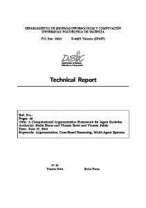
Figure 2.8: Peppytide model assembly. (a) Bore dimensions and assembly plan for the amide unit and α−carbon unit joint (cross-section view drawn to scale); the same scheme was used for the Cα − CH3 joint. (b) Representation of a hydrogen bond between distal amides. (c) A Peppytide homopolymer (polyalanine); black part, amide unit; white part, Cα unit; blue part, methyl group unit; red ring, oxygen; white ring, hydrogen; blue dot, nitrogen.
33
2.3.5
Long-range interactions The representation of hydrogen bonding is another important feature reproduced
in the Peppytide model. The long-range hydrogen bond interactions of the polypeptide chain are key to formation of the secondary and tertiary structure. The model reproduces the hydrogen bond donor (NH group) and acceptor (C=O group) behavior of distal amides by using a pair of rod magnets (Figure 2.8b). Magnets are a reasonable approximation of the hydrogen bond interaction because in reality the NH and C=O groups attract each other but not themselves, similar to the north and south poles of a magnet. Importantly, this feature allows the model to reproduce long-range interactions between monomers that are separated in sequence space, yet are in close contact in 3D space, thus enabling and stabilizing secondary structure. Previously, Olson’s articulated polypeptide chain model has demonstrated the use of magnets as hydrogen bonds [19]. Magnets are only an approximate means to represent the H-bond interactions, as the force-distance relationship in magnets is different from that of H-bond strengths. Although both have exponential decay rates, the H-bond strength [42] exhibits a different decay rate than magnet-array fields [43]. However, their decay curves follow roughly similar trends, making the magnets a practical choice for representing H-bonds approximately. Another advantage is that they are passive components requiring no power to operate.
2.4
Model assembly The parts of the model were 3D-printed and assembled into a chain. This
section provides a step-by-step guidance on assembling the model. Further information 34
about assembly can be found in the published sources and the Peppytide website [1, 44, 45]. All of the three units of the model were designed to be hollow to make them as light as possible to minimize the impact of gravity. The parts were created using a 3D printer using acrylonitrile butadiene styrene (ABS) plastic. The 3D-printable stereo lithography (STL) files for these parts are provided to enable anyone to readily produce the Peppytide model themselves (Appendix A). Undersized pilot holes are designed in each part to guide drilling precision bores for the bond pieces and magnet installation. The parts were subsequently assembled in a chain using cheap screws and spacers (Figure 2.8a, Appendix B). The Peppytide model can be assembled using the following steps: Step 1: Part printing. 3D-printing of 3 types of units as described above: amide, alpha-carbon, methyl-group (printing, soaking, drying). (see supplementary STL files for the parts, Appendix A). See Appendix B for details on magnets, screws, spacers and nuts needed for assembly. Step 2: Amide unit preparation. a. Installation of the H-bond magnets. Sand the bottom face of the H-bond magnets (3/16�� ×1/8�� ) with 220 grit sandpaper to roughen the surfaces for effective adhesion. Next, glue the magnets onto the amides using Epoxy (JB-weld); O with North pole up; H with South pole up (Figure 2.9). Leave for 24 hours for setting and drying. b. Labeling. Color-code the amide units with red-ring for oxygen, white-ring for hydrogen, and with blue-dot for nitrogen atoms in the amide units (Figure 2.9).
35
c. Drilling dihedral rotational barrier magnet holes. Enlarge the magnet holes by drilling to a depth of 0.074�� (drill size #31, 0.120�� ) in the amide units (see Appendix C for detailed drilling dimensions). This hole-depth will allow each magnet to protrude by ∼ 0.051�� . Slightly undersized guide holes are provided to minimize the amount of material removed by the drill. d. Drilling the bond holes. Enlarge the central bond holes (C and N atoms) by drilling to a depth of 0.345�� (drill size 0.250�� ) in the amide units. This hole-depth will allow the nylon bond spacer to protrude by 1/32�� . Slightly undersized guide holes are provided to minimize the amount of material removed by the drill.
Figure 2.9: Steps of assembly: Amide unit.
36
Step 3: Alpha carbon unit preparation. a. Drilling the rotational barrier magnet holes. As with the amides, enlarge the magnet holes by drilling to a depth of 0.074�� (drill size #31, 0.120�� ) in the alpha carbon units. This hole-depth will allow each magnet to protrude by 0.051�� . The final bore diameter of 0.120�� is intentionally undersized to allow a press-fit of the 1/8�� diameter magnets (see step 4 below). b. Drilling the bond holes. Drill to a depth of 0.300�� (drill size #43, 0.089�� ) on the 3 faces (N-face, C-face and the side-chain-face) of the alpha-carbon units. Guide holes are provided, by design (Figure 2.10). c. Tapping the bond holes. After drilling the central bond holes, tap them with 4-40 threads to their full depth (Figure 2.10).
Figure 2.10: Steps of assembly: Alpha carbon unit.
Step 4: Addition of the rotational barrier magnets. Press fit the dihedral 37
magnets (1/8�� ×1/8�� ) into alpha carbon units (with North pole up) and in amide units (with South pole up). Step 5: Bond linkage assembly. Assemble screws, nuts, and spacers for bond linkages (Figure 2.11 left). There are 3 such bonds per monomer unit: Cα –Amide(N), Cα –Amide(C), and Cα –Side-chain.
Figure 2.11: Steps of assembly: Assembled bonds and related parts that need to be linked per repeating monomer unit.
Step 6: Alpha-carbon bond assembly. Assemble bonds into the Cα units by screwing the bonds into the alpha carbon and securely tightening the nut, while leaving a slight gap to allow free rotation of the spacer (Figure 2.12).
38
Figure 2.12: Steps of assembly: Alpha carbon unit with bond linkages.
Step 7: Backbone assembly. Push-fit bond linkages from Cα units into amides (Figure 2.13). The bonds will bottom out into the amide bores.
39
Figure 2.13: Steps of assembly: Connecting the alpha carbon unit with the two faces of amide units.
Step 8: Repeat steps 6 and 7 to make the entire backbone chain of alternating amide unit and alpha-carbon unit (Figure 2.14).
40
Figure 2.14: Assembling backbone
Step 9: Adding side chain residues. Lastly, press-fit the methyl groups onto the 3rd bond linkages of the Cα units in the backbone chain (Figure 2.15).
Figure 2.15: Final assembly of side chains
Step 9 gives the final assembled Peppytides chain. Step 10: Begin Folding experiments. Now the model is completely assembled and ready for trying folding with it. To initiate the folds of an alpha-helix, the template in Figure 2.16 is used. More details on folding process can be obtained from the movie in 41
Appendix E.2 and from Peppytide website [45].
Figure 2.16: Helix Template
2.5
Alanine di-peptide: The smallest peptide Alanine di-peptide is the smallest peptide possible, with 2 amino acids and a
peptide bond (amide) holding them together. Based on the above design of the units, the simplest assembly that contains both φ and ψ bonds is an α−carbon unit linked to two amide units. This forms an amide-Cα -amide arrangement in the model that we refer to as an amino acid diamide (Figure 2.4a). For a longer chain assembly, Figure 2.8c shows a generic polypeptide chain physical model.
42
Figure 2.17: Alanine di-peptide
2.6
Scale of model The Peppytide model (Figure 2.8c) is approximately 93,000,000 times magnified.
As mentioned in Section 2.3.2, the scale factor of Peppytide is 1˚ A = 0.368�� . This scale was chosen so that the model is big enough to hold all the screws, nuts, spacers and magnets, while small enough for each part to be operated by hand easily for folding. The weight of the model was also a constraint. We aimed to keep the model as light as possible. For this version of the model, a 9-mer poly-alanine model weights about 140g. A 9-mer chain can be folded into a 2.5 turn α−helix. More details about the weight measurements can be found in Appendix B. The advantage of having a precise scale-factor is that the model can be physically folded with hand, measured with a ruler, and then converted to the corresponding ˚ A value to get the dimension of the folded structure at the atomic scale. We have tested that this method works well in folding of α−helix, β−sheet (Sections 3.1.3 and 3.1.4). Thus, the
43
Peppytide poly-alanine is 1.3 × 10²³ times heavier than its biological counterpart, and is light enough to be manually folded into secondary and tertiary structures.
2.7
3D printing an entire model In the above sections we discussed how to 3D-print the Peppytides and assemble
it. However the assembly process has a lot of steps and is quite complex. Though this gives us precision, often (and especially to beginners) it is desirable to have a version that is easier to make. For example, I have received a request where the instructor wants to just 3D-print multiple models and distribute it to the classroom without the hassle of the assembly. To cater to this audience, we have designed a version of the model that will print an entire chain in a single 3D-print run. With our printer capability, currently we are able to make up to a 7-mer, but it is possible to optimize the design to print longer chains. With a compact conformation that unfolds after 3D-printing, it should be possible to print up to a 80-mer or 90-mer chain in a 10cm × 10cm × 10cm space inside standard 3D-printers. The methodology for this kind of optimization already exists where a very long 1-dimensional chain is printed within the small confines of the 3D-printer and which unfolds after the supporting material is removed [46]. Foldable jewelry and accessories were also printed with similar methodology of physical “zipping” [47]. The shortcoming of this version would be the lack of dihedral angle preferences as we will not be able to install the magnets, but it will have all the other features including the flexibility of backbone, the degrees-of-freedom and the hydrogen bonds.
44
2.8
Designing for specific proteins We have discussed the design of a generic polypeptide chain model, which was
implemented by placing the dihedral magnets based on the calculated average preferences of φ and ψ for all such angles along the chain. Extending this concept, it should also be possible to create a model with assignable and distinct bond angles for each backbone dihedral angle, which would bias them to fold into a pre-determined structure. These models are expected to fold making pre-determined conformations, which would serve as an useful tool for structural biology as each of these dihedrals will be biased to make the same structure every time it folds. To make a specific model of a peptide with preassigned sequence of the φ/ψ angles, we can position the magnets at precise locations, unique to the values in this sequence, by varying the locations of these magnets as we go along the chain. Because of its customizing nature, it is essential to build an application that would output user-defined customized chain ready for 3D-printing. More details in Chapter 4 shows how we are automating and optimizing the design for such applications (Section 4.4).
45
2.9
Summary In this chapter we explored the feasibility of Process 3. We have looked at the
design of a generic physical model of polypeptide chain and its assembly. We have also discussed the work-in-progress for building side chains and design towards making specific structures. We have made the design of the model open-source to encourage people to make their own proteins models. In Chapter 3 we proceed to discuss how to make biologically relevant structures with them.
46
Chapter 3 Folding with Physical Models
3.1 3.1.1
Folding in Peppytides Why physical models to study folding? Folding of Peppytide, the physical model of the polypeptide chain, serves as a
proof-of-concept that a bijective mapping can exist between the physical model and natural proteins. That is, both Process 3 and Process 4 are feasible. We have explored Process 3 in Chapter 2. Here we explore Process 4, that is, how accurately the physical model represents natural polypeptide chain behavior through folding (Figure 3.1). As discussed in Section 1.3 this serves as the proof-of-principle that because of this accuracy in folding, a mapping should also exist between the physical model and the computational models. The proof serves as the connecting dot to validate the existence and 47
Figure 3.1: Exploring Process 4: From physical models to natural proteins
utility of the computational space at the intersection of N, C and P, which is the core concept that this dissertation establishes. Thus this chapter serves as the basis for the physical-digital platform development and computational interfacing discussed in Chapter 4.
3.1.2
Which folded structures we explored and why? The question that comes to mind is whether by testing a finite set of folds with
Peppytides would provide sufficient grounds to the claim discussed above. Is the search thorough enough? Does it cover the full set of possibilities in order to claim that Peppytide can serve as an accurate macro-scale polypeptide macromolecule with all its dynamics? What are its limitations?
48
To answer these questions, we travel back to the Ramachandran plot (Figure 2.5) and enlist all the possible folds that are most frequently evidenced in natural proteins. Accordingly, we test the model with an exhaustive set of secondary structures, and a few small tertiary structures and common motifs. These folds are tested for accuracy, dimension and stability after folding. We tested the model by folding it manually into a variety of secondary structures. The right-handed helices that we made are the ubiquitous α−helix, and the less frequent 310 helix and π−helix. Left-handed helices are not so common in nature. We made the parallel and anti-parallel β−sheets, the two types of possible β−sheets. We made the β−turn types frequently found in nature. For tertiary structure, we made the ββα motif, one of the most common motifs found in proteins, and a small protein, Osteocalcin, found in bones of animals. We compared the model structures with those of the analogous crystal structures of proteins found in nature (Sections 3.1.3 and 3.1.4). Supporting Movie in Appendix E.2 shows how Peppytide can be folded into an α−helix and an anti-parallel β−sheet (also see Appendix E, Movie E.1).
3.1.3
Folding and measurement of α−helix The right-handed α−helix is one of the most frequent secondary structure found
in proteins. It has been extensively studied since Pauling’s discovery of the structure in early 1950s [16]. The structure is formed and stabilized by forming a hydrogen-bond between every i → (i + 4) amino acids. 49
In Peppytides, we can see these hydrogen-bonds being formed between the respective amides due to the H-bond magnets incorporated in the model (black parts in Fig. 3.2 b and c). Due to the backbone flexibility, the process of manual folding of the helix is effortless with some practice. A folding template has been designed for Peppytides to aid in the folding process, which stabilizes the first 3 hydrogen-bonds in the chain (seen in Fig. 2.16, and in use in Fig. 3.2c). This process is the equivalent of the helix initiator process in vivo where a helix initiator protein aids in the first fold formation of α−helix. The α−helix, measured over 3.5 turns (measured from the α−carbon of residue 1 to the α−carbon of residue 13) in the Peppytide, is 6.78�� ± 0.16�� (equivalent to 18.43 ± 0.45˚ A with scale factor of 1˚ A = 0.368�� ), which is in excellent agreement with an α−helix of same length measured at 18.4˚ A in the protein structure (pid:2ZTA chain B) (Fig. 3.2 a and c).
50
Figure 3.2: Peppytide folded into α−helix, a secondary structure.
Comparison of a
13-mer polyalanine α−helix (RM = 0.7RV DW ): (a) α−helix from crystal structure (from leucine-zipper pid:2ZTA, residues 16-28) (Upper: front view; Lower: top view); (b) Peppytide in CAD reconstruction, the computer-representation with theoretically ideal values of φ = −62°, ψ = −42°; (c) Peppytide physical model. Alanine side chains are in red for (b) and (c).
51
3.1.4
Folding and measurement of β−sheets The parallel β−sheet measured in the Peppytide over five amides in each of the
two strands (measured from the nitrogen of amide 1 to the nitrogen of amide 5 in the same strand) is 4.85�� ± 0.04�� (equivalent to 13.20 ± 0.12˚ A with scale factor of 1˚ A = 0.368�� ). This agrees well with the parallel β−sheet of equivalent length in protein structure as 13.4˚ A and 12.9˚ A on the two strands (pid:202J, chain A). Figure 3.3 shows two strands of the model chain in parallel and anti-parallel conformations.
52
Figure 3.3: Peppytide folded into β−sheets. Two strands of polyalanine Peppytide model folded into β−sheet conformations (with blue alanine side chains in one strand, and red in the other strand): (a) anti-parallel, (b) parallel; the views to the Right show the natural curvature of the sheets.
The β−sheets made with the Peppytide model have a natural curvature as found in protein β−sheets.
53
3.1.5
Folding of β−turns β−turns are one of the most commonly found secondary structures in proteins.
We made type I and type II β−turns with the model, and compared them, respectively, with the type I β−hairpin turn found in ubiquitin (pid:1AAR, turn-seq:TLTG) [48], and the type II turn found as a subpart of the β−barrel in factor H binding protein (pid:3KVD, turn-seq:GSDD) [49] (Fig. 3.4 A and B respectively). Protein β−turns often contain a glycine at the R2 or R3 position [50]. All of the side chains faced outward, so it was not a problem to form the folds in the model.
Figure 3.4: Folded β−turn secondary structures, types I and II, formed with the Peppytide model. (a) type I in Peppytide compared with a turn in pid:1AAR, residues 4-14. (b) Type II in Peppytide compared with a turn in pid:3KVD, residues 221-228. 54
To facilitate folding into the various turn conformations, the side-chain methyl group in Peppytides can be removed to create a glycine residue. β−turn types I, I� , II, and II� were constructed with a glycine version of the model (Figure 3.5) based on existing turn angle values [51]. Type I� and type II� are more common in β−hairpins found in nature [52– 54]. Interestingly, these turns once formed in Peppytides had a tendency to shift their conformations to attain a greater stability. For example, the β−turn type I and II models showed a propensity to revert to their more stable counterparts, the type II� and type I� turns, respectively. All the turns could be folded with obstruction in the model even though the values of φ and ψ for the turns are different from those enforced by the magnet arrays. This was because the turns were stabilized by a combination of the conformational constraints imposed by both steric interactions and the hydrogen-bonding magnet interactions.
55
Figure 3.5: Type I, I� , II, II� β−turns made with Peppytide. (a) Type I, (b) Type I� , (c) Type II, (d) Type II� . (Left) Top-view of Peppytides parts assembled in CAD software to form β−turns. (Center) Front-view of Peppytides parts assembled in CAD software to form β−turns. (Right) β−turns made with the model.
56
3.1.6
A comparison between 310 helix, α−helix and π−helix
Figure 3.6: A comparison between 310 helix, α−helix and π−helix
3.2
Tertiary structures With longer Peppytide chains, we have successfully folded it into several known
protein conformations. These are minimal structures as the side chain space-filling effects 57
have not been taken into account – the model consists of only alanine side chains. However in a future study, it would be interesting to compare and contrast the structures with and without the correct side chains to study the effects the side chains can have in converging to the least-energy configurations. We have assembled a 28-mer chain to fold into the tertiary structure ββα motif (pid:1FSD) [32] (Figure 3.7).
Figure 3.7: Protein structural motif with Peppytide model.
(a) De novo ββα motif
(pid:1FSD), a 28-mer; blue side chains indicate N-term; (b) protein ribbon structure, green indicates loop and β−sheet, and red indicates α−helix.
58
We made a 45-mer chain to fold into fish osteocalcin (chain A; pid:1VZM). Fig. 3.8 shows that Peppytide is capable of being folded into complicated structures due to longer chains.
Figure 3.8: Tertiary structure of Fish Osteocalcin (chain A), a bone protein with 45 amino acids (pid:1VZM); blue side chains indicate N-term; (right) protein structure cartoon, green indicates loop, and red indicates α−helix.
3.3
Discussion Because of the combined stabilization of each local dihedral angle and the longer-range
hydrogen bonds, Peppytides can form very stable secondary structures quite easily. The β−strands in the model can be formed with very slight human intervention with just light shaking of the chains, when the model attains the minimum energy positions, and can be 59
easily converted into parallel or anti-parallel β−sheets, or β−turns (Figs. 3.3 and 3.4). The α−helix can be easily formed with the help of a template (that can double as a stand) that facilitates the “nucleation” of the helical fold (Fig. 3.2). Once formed, the model helix is very stable to external stress/strain. We have tested the ease with which the model can be folded into an α−helix and β−sheet with the kids at the Lawrence Hall of Science Museum at University of California, Berkeley, as described in Chapter 5. All secondary structures made with the model are very stable to handling due to the combined stabilizing effects of the H-bond magnets and the rotational barrier magnet arrays. The strength of the H-bond magnets (pull force, 2.49 lbs.) was chosen to overcome the effect of the model weight and hence the influence of gravity, while still forming stable H-bonds (Appendix B). The H-bond magnets have been designed to touch and form the CO· · · HN bond based on the standard O–N distance in polypeptides. For two distal amides forming a hydrogen bond, the O–N distance is typically 3.00 ± 0.12˚ A, from α−helix crystal structure (pid:2ZTA). In the Peppytide model, the O–N distance is 1.17�� ± 0.04�� (equivalent to 3.18 ± 0.11˚ A).
3.3.1
Backbone flexibility The models were successfully folded into all types of helices found in proteins,
from the tightest i → (i + 3) 310 helix to looser i → (i + 4) α−helix to loosest i → (i + 5) π−helix. This demonstrates that the model is able to withstand the twisting and folding
60
flexibility needed to exhibit the entire range of polypeptide backbone dynamics. The longer chain folds illustrate that the model has the capability to make meaningful polypeptide tertiary structures of small but considerable length in which to explore various structures and their intermediates.
3.3.2
Unfolding of the α−helix to β−sheet in Peppytides Unfolding of the α−helix has been widely studied, both experimentally [55] and
computationally [56]. It is an important problem to study. It is thought that the onset of neuro-degenerative diseases in many cases are due to misfolding of proteins to form β−amyloids [57, 58]. α−helices have been known to undergo transformation into β−sheet under mechanical pressure, and is especially relevant to amylogenic diseases. Thus any tool to study the unfolding process of α−helix would be of great value to the research community. To test the unfolding of the α−helix manually, we applied mechanical pull directly along the helical axis. Pulling in the direction of the helix axis does not unfold the helix easily. However, with the application of a slight unwinding torque (along the helical axis) on both sides, unfolding starts readily at the termini and gradually proceeds inward (Figure 3.9).
61
Figure 3.9: Transition of α−helix to β−sheet in Peppytide due to an applied torsional unraveling force on both sides.
62
3.4
Advantages of folding a customized model over generic model The structures studied in this chapter demonstrate that a generic Peppytide
chain can readily adopt a variety of specific folds accurately and to-scale. In future we will be able to make on-demand foldable models of proteins based on crystal structures. We will be able to fold these custom-made models into particular proteins to study their structures and be able to manipulate these structures with hand. From the point-of-view of folding, a big advantage of the specific chains, over the generic, is that the dihedral magnets would be positioned to choose one particular angle for each specific phi and psi in the sequence. Thus, in combination with side chain additions, it will be easier to study minor fluctuations in structures or mutations. We will create models where each dihedral angle is confined to a specific value. In Section 2.8, I explained the design considerations of these models. There is scope to further enhance the performance of the customized physical models by focusing on precise designing and optimization. In Section 4.4, I presented a digital platform workflow through which anyone can design, simulate and make their specific proteins. We aim to simulate the effect of positioning the magnets to optimize the preference for the native configuration. Thus, we are on the verge of making it possible for everyone to make extremely complex structures of proteins on a regular basis, the folding of which will be highly instructive to the researchers. With the leaps in 3D-printing technologies every year, the day is not far when we shall be able to print entire proteins with atomistic details that will be foldable. 63
3.5
Summary In this chapter we have explored the feasibility of Process 4 through various
secondary and tertiary structures of proteins using the generic Peppytide model. We made measurements with the model and compared it with crystallography structures. Hence we concluded that the model can be folded into all the possible secondary structures found in proteins. We have also established that it is a precisely scaled model. Hence, folding a structure with the model, followed by measuring with a ruler and converting to nano-scale, would essentially measure the corresponding nano-scale structure and its dimensions. This flexibility provides grounds to form a bijective mapping between the physical model and its digital representation that we discuss in Chapter 4.
64
Chapter 4 Towards a Computing Paradigm for Physical Biomodels
The state-of-the-art molecular dynamics techniques for protein folding involves simulation of biological systems for analyzing minimum energy configurations. Though simulations provide a successful and precise means to study the phenomenon, they still lack a platform that will facilitate an intuitive understanding of the underlying complexity. On the other hand, the form-specific, scaled physical model that we have prototyped brings forth the possibility of direct manipulation with hand. There is a need for a ‘glue’ that will tie the physical and the digital together, complementing each other through intuition and precise computation. A new paradigm emerges from this philosophy that brings together Implementation of the Peppytide-digital representation is done using Project Cyborg from Autodesk, Inc. in collaboration with the Bio/Nano/Programmable Matter Group at Autodesk, led by Carlos Olguin. More information about Project Cyborg is available at [59]. 65
the best of both worlds. The ultimate goal is to drive structure information back and forth from computational to physical models and vice versa. This paradigm sets forth new ways to think about bio-macromolecules. While Chapter 2 discusses the design methodologies and the parametric considerations that we have made for the physical model, Chapter 3 shows the prototype being used successfully to emulate the shape and mechanics of polypeptides (Process 3 and Process 4 respectively). With this foundation, we envision a platform where the computational and physical models complement each other in order to provide an enriched knowledge base for intuitive structural analysis of proteins. We explore these relationships in this chapter with Processes 5 and 6. A mapping of the physical model to its digital counterpart ensures a two-way interaction between the physical model and its digital representation. The digital representation can then be generalized, parameterized, and optimized for specific functionality to make specific 3D-printed physical models (Process 5) (Figure 4.1). We achieve this by volumetric CAD representations of the constituent parts tagged with angle and location information, and parameterizing them.
4.1
A brief history of the physical-digital space The concept of Pervasive Computing, with physical objects involving hidden /
embedded computing capability, has been stretched to the limit and are being explored further as we speak [60–62]. A lot of research and industry efforts have been made in
66
Figure 4.1: Exploring Process 5: From computational models and CAD to physical models
the fabrication of “smart” objects at the interface of the physical and digital world in the form of Tangible User Interfaces [63, 64], wearable computers like Sixth Sense and Google Glass [65–67] and smart sensors [68, 69]. There has also been the reverse flow from the physical to the digital world in forms of 3D User Interaction (3DUI), Virtual Environments & CAVE-technology (Computer Aided Virtual Environments), and haptic input devices [70– 72]. A few other examples of explorations on input/ output devices are ClearBoard [73], Tangible bits [74], Triangles [75], WebClip [76] that tie together digital bits and physical manipulatives. Recently with the advent of 3D printing technology, there has been a revolution in the design and manufacturing of prototypes in art and technology. It catalyzed the ideation and realization of concepts ranging from art, architecture and design [77, 78] to tissue printing [26, 27]. Further, with the availability of the easy-to-hack Arduino boards, 67
LilyPads and other hardware prototyping units, a series of research directions have emerged with enriched user experience in mind. With rise in cutting edge camera technology and gesture analysis, interesting gaming platforms and internet-based applications have emerged that has proved to be trend setters in consumerism. Over the last two years, Microsoft Kinect technology have garnered a lot of interest in game development through skeletal tracking [79,80], and object recognition through computer vision [81]. Research has also been done with simple webcams and mini-projectors for gesture recognition and to interact with the physical world [65]. Some of these technologies have been able to produce meaningful information for visualizations in biology problems. For example, pressure-sensitive haptic devices have been used in combination with molecular graphics [82], for experiencing variable molecular forces through torque-feedback [83, 84], for docking between proteins and ligands [85]. The CAVE technology was invented with scientific visualization in mind. Biomedical data visualization with immersive CAVE and CAVE2 are being explored, where the audience is immersed in the visualization-space and can walk around the projected 3-dimensional object [86, 87]. People can look around from every angle or underneath, and can have a feeling of touching the object, or a feeling of being inside the object. With all these advancements in tools and technologies made over the last few decades, we are at the cusp where physical biomodels can not only be haptic or other input devices or manipulatives, but can also contain and convey information by virtue of its physicality. They will have a seamless flow between the digital and the physical. We envision that such models and devices will be able to contribute to computation by virtue of its form, orientation and motion.
68
4.2
The concept of a physical-digital paradigm for biology Though the current developments have influenced different modes of computing
like Gaming, Social Computing and Human-Computer Interaction (HCI) as seen above, there are very few developments at the biological-digital interface at macro-scale, or for any other type of compute-intensive simulations for scientific discovery having a tangible counterpart. So far, this type of interfaces have been only used for interaction, story-telling, information access and visualization. But never has the physicality, shape and orientation of the real-world objects been the site or source of computation within biomodeling tools. Some experimental studies have been made in biology with augmented reality, but in these cases all computations happen in the computer itself while the tactile devices serve as manipulatives. In this chapter, we explore the feasibility of the physical-digital interfacing of Peppytide as preliminary proof-of-concept for the structure and orientation of real-world objects adding a computational dimensionality. As a first step, here we present a platform for easy customization of physical models of polypeptides enabled by the ability to modify a few parameters in the CAD design cycle of the physical model. At the end of the optimization cycle, these precise CAD representations serve two purpose: (1) in 3D printing an accurate physical model, and (2) as an input to the digital representation of the physical model. This approach has the advantage of enabling easy and precise bijective mapping between the physical and the digital counterparts of the same artifact (Figure 4.2).
69
Figure 4.2: Physical model and digital platform
4.3
A methodology for the physical-digital paradigm for polypeptides at nano-scale There are three steps involved in the process of making a bridge between a
physical object and a computational platform for polypeptides: (1) to have a digital representation of the physical model that embeds its properties, (2) to provide a digital computational 70
environment within which the digital model might function, and (3) find the best way to track the physical model and its dynamics. At present, we focus on the first two steps. Our work targets a seamless interactive modeling and computing environment between Peppytides and an emerging biocomputational tool, Cyborg (Section 4.3.4). The goal is to have a digital representation of the physical version of Peppytides that will enable physical-digital interfacing. For a better design of the physical representation of the polypeptide, we are simulating the physical model itself to take into account the influence of magnet strengths and gravity, and to study the folding pathway (i.e. a step-by-step guidance of the folding sequence over time) in two ways – the way a user might fold a Peppytide, and the way a protein might fold temporally at nano-scale. This approach not only can focus on the way a protein might fold itself at nano-scale, but also the steps people would take to fold a chain model that is 100 million times magnified with issues like gravity, coarse-graining and impractical interlocking of components. With this work we aim to quantify how closely the physical model emulates proteins.
4.3.1
Biomodeling platform for Peppytide digital representation: The Peppytide API We have designed a web API (Application Programming Interface) platform
where users can design their own physical model of polypeptide, and 3D-print the parts for final assembly. This is possible because of the digital representation serving as the underlying knowledge base at its core. It enables an easy conversion of the design principles
71
of CAD-oriented modeling to biological macromolecules (polypeptides) and vice versa. This prototype is a proof-of-concept that marrying CAD-based platforms and 3D-printing with biocomputational simulations opens up new possibilities for research in biology. Within this platform, we hope to be able to digitally fold, unfold, and assemble the physical-digital model using self-assembly simulations. This feature will serve useful purposes for users who would like to: (a) 3D-print and assemble a physical polypeptide model, and (2) simulate the behavior of the physical model using a back-end solver, Nucleus, so as to take into considerations its physical parameter constraints like weight and magnet strength. We use Cyborg, the CAD-enabled biocomputation framework developed by Autodesk Inc., with software features and modeling languages to program the digital model that will be a representation of our physical model. More details about Cyborg and Nucleus are in Section 4.3.4.
72
73
Figure 4.3: Peppytide workflow and UI mockup-design in Cyborg. [Autodesk screen shots reprinted with the permission of Autodesk, Inc.]
Storing data.
The user data corresponding to the application is stored in a remote
repository. The data is pulled from this repository every 2 minutes to update our application server.
4.3.2
Digital representation: Simulating the physical model
The digital representation consists of three parts:
1. B-rep – For a visual representation we use the standard boundary representation format (B-rep) from solid geometry. It is a computational geometry solution that ties together the constituent CAD subparts. It is a CAD solid modeling technique to represent a objects in terms of surfaces and faces. This format is used in producing views in the application. 2. Orientation – A matrix consisting of the positional information of the parts in sequence. 3. Parameterizing – The faces of the subparts are to be tagged in the B-rep in order to parameterize certain factors in the geometry to enable higher-level customization. An application of this design consideration is in making specific protein models with precisely located magnets.
74
Figure 4.4: The design of workflow for implementing physical-digital Peppytides through the Cyborg platform.
4.3.3
The workflow for digital-physical interfacing of Peppytides The main operation performed by the API described in Section 4.3.1 can be
summarized with a workflow outlining the information flow from user input to the 3D-printed model (Figure 4.4). This workflow converts a sequence of amino acids through user-input into the corresponding digital representation of the physical model. In this scheme, the amino acids are broken up into alternating copolymers of amide and alpha-carbon units along with the respective side chains (see Chapter 2 for details).
75
A second way to define the sequences is by drawing and connecting the parts directly using tools from the “Parts library toolbar” instead of inputing the sequence. This mode of input will in turn update the amino acid sequence field. This mode was added to the workflow to provide a smooth learning curve to the non-specialists about the structure of polypeptides, and also to provide a quick way for specialists to edit an existing model diagram in the GUI. We have defined a grammar described in Section 4.5 to constantly check the validity of the interconnectivity between parts. We have used the standard .OBJ file format, a 3D object file format, to contain the digital representations of the parts of the physical model. It is a data-format for 3D geometry in terms of vertices, faces, and textures of faces. The parts library consists of the following 3D-CAD parts: (a) the two main chain parts, amide and alpha-carbon units, (b) the two end-terminal parts, N-terminal and C-terminal, and (c) all the side chain parts. All parts are in .OBJ file format which is then imported into Cyborg’s internal data structure. The goal of this workflow is to generate a production-quality CAD-cum-biocomputation service wherein Peppytide representations of any given protein of interest could be automatically generated, and the parts be 3D-printed, to allow any interested party to make and fold their own proteins.
76
4.3.4
The Cyborg and Nucleus Autodesk platforms Project Cyborg (www.autodeskresearch.com/projects/cyborg) is a web-based
platform developed by Autodesk, Inc. to provide cloud-based computation along with CAD functionality for programming matter across scales [59]. This design of the platform enables researchers and developers to develop their own domain-specific platforms and applications. Cyborg’s main focus is in biology-based applications with domains stretching from nano-particle design to tissue engineering to human-scale self assembly. Nucleus is another project by Autodesk, Inc. It is a universal solver for dynamics of objects, and can handle motion of bodies at any scale [88]. It has a core physics engine that can be used to simulate physical effects in our models, like weight, magnetic field, and flexibility. We are simulating the self-assembly of polypeptide chain backbone with it and exploring folds of the macroscopic physical version of polypeptides.
4.4
Parameterizing to enable design of specific proteins The amide and the alpha-carbon units are connected at the phi and psi faces. For
prototyping the generic polypeptide chain, we put magnets at the most-preferred, average angles on these faces in order to bias the phi and psi angles, that is, to add rotational barriers as found in native protein structures (Figure 4.5). To make a specific protein, as opposed to this generic design, the position of magnets can be optimized to account for that particular value of phi or psi and other variables
77
Figure 4.5: Rotational barrier for generic polypeptide backbone. (a) phi-face, (b) psi-face.
78
like weights of parts and strengths of magnets. The advantage of such an optimized design is that we will now be able to make particular chain that is predisposed to fold into one specific conformation. In this scheme, it is essential to store the phi and psi values for each position along the sequence. The node-graph for the polypeptide model sequence contains the phi and psi values and sequence number, seqNumber, for each node as shown in Figure 4.7. The .OBJ file information is obtained from FilePath that accesses the parts library. These .OBJ files are tagged with the position of the magnet holes on the faces of each part. We can parameterize these hole positions and automatically put a magnet-hole within the solid geometry of the parts based on the angles phi and psi for that particular amino acid in that particular position in sequence. Thus, the generic geometry of parts obtained from .OBJ files will be updated resulting in slightly different 3D drawings done programmatically. Each of these parts is abstracted within a node N-Term, Alpha-Carbon, Amide, Alpha-Carbon-1, Amide-1 or C-Term. As a result of these operations, the main workflow (top one in Figure 4.6) will output an array of similar parts with different magnet hole positions. These array of parts can then be processed to be converted to 3D-printable files. To define the overall structure of the polypeptide chain, each part will also have the translation and rotation variables. This position data is essential for generating a CAD-cum-PDB file format for the digital model (details in Section 4.8). Once we generate this file, simulations for self-assembly can be performed on the digital model. The side chains play a major role in protein folding. To account for specific
79
amino acid side chains in each position, each Alpha-Carbon node facilitates the specification of different side chain functional groups through side-chain. Addition and editing of side chain properties (type, sequence#, translation and rotation) can be handled through the API dashboard cassette (seen at the bottom in Figure 4.7). This dashboard also allows addition of other types of nodes as per user need.
80
81
Figure 4.6: The parameters for the main workflow and the digital representation; N: N-terminal, C: alpha-Carbon-Unit, A: Amide-Unit. [Autodesk screen shots reprinted with the permission of Autodesk, Inc.]
82
Figure 4.7: The parameters for the digital-physical representation. [Autodesk screen shots reprinted with the permission of Autodesk, Inc.]
4.5
A grammar for model checking of backbone In a platform in which users have free reign on design of a system by manipulating
in GUI (Graphic User Interface), it is imperative that a set of model checking rules need to be implemented to verify the model being designed. To keep it biologically relevant for polypeptide chains, the platform needs to have a model checking running in the back-end. It needs to be incorporated in the workflow so as to have a seamless design experience for the users. The following grammar has been implemented to check for the accuracy of the proper digital assembly of the polypeptide backbone so as to represent the amino acids correctly. Figure 4.8 shows a graphical representation of the grammar. Start → N -term · A | � A → C-alpha · B B → Amide · A | End End → C-term With this grammar, we can generate the following chains:
• Empty (null) chain: � • 1 amino acid (AA) chain: (N -term · A) = N -term · (C-alpha · B) = N -term · C-alpha · (End) 83
= N -term · C-alpha · C-term • 2 amino AA chain: (N -term · A) = N -term · (C-alpha · B) = N -term · C-alpha · (Amide · A) = N -term · C-alpha · Amide · (C-alpha · B) = N -term · C-alpha · Amide · C-alpha · (End) = N -term · C-alpha · Amide · C-alpha · C-term • 3 amino AA chain: (N -term · A) = N -term · (C-alpha · B) = N -term · C-alpha · (Amide · A) = N -term · C-alpha · Amide · (C-alpha · B) = N -term · C-alpha · Amide · C-alpha · (Amide · A) = N -term · C-alpha · Amide · C-alpha · Amide · (C-alpha · B) = N -term · C-alpha · Amide · C-alpha · Amide · C-alpha · (End) = N -term · C-alpha · Amide · C-alpha · Amide · C-alpha · C-term • And so on · · · Thus, with this grammar we can generate amino acid chains of any length by expanding the non-terminals as necessary. As this chain growth has definite directionality, it will prevent any other type of connection between the 4 types of parts N-term, C-alpha, Amide, C-term, thus preventing all other non-AA type combinations.
84
Figure 4.8: A graphical representation of backbone grammar
4.6
Capturing physical model with camera: From physical model to digital form A natural next-step would be to capture the structure of the physical models
which can then be represented digitally in real-time (Process 6, Figure 4.9). To capture the images and motions of the physical model, we need a camera that can take images with a minimum speed of 25 frames per second. In order to get a 3D digital image, we need to have depth perception feature in the camera. We plan to have the camera talk to the computer, where the images can be analyzed for further computations. Object recognition algorithms will be implemented to recognize the position of alpha-carbon atoms in the physical models, and then to reconstruct a digital model based on these positions, much like the computational geometry algorithms used for NMR data for determination of protein structures. Similar kinds of object tracking experiments have been made with lego blocks where a Microsoft Kinect camera, with depth-sensing feature, tracks the building up of an object from constituent lego parts [89, 90]. 85
Figure 4.9: Exploring Process 6: From physical models to computational models
A software tool that captures the structure of physical models from camera can be developed as in Figure 4.10. Also, this digital structure can be ported to a format (for example, pdb) that can be used by other softwares to make useful computations, simulations and predictions. Furthermore, augmented and Virtual Reality user interfaces can also be made to get better user-oriented protein structure visualization in 3D in space, as explained in the next section.
4.7
Augmented reality and virtual reality in biology The techniques in Augmented Reality (AR) and Immersive visualization have
been explored in biology in the past to enhance user experience. In AR a manipulative object is used to maneuver digital data. Tangible models have been used to study enzymes 86
Figure 4.10: Physical model as input device. and corresponding electrostatic potentials, where the camera traces an embedded pattern used as a marker in the tangible model [3]. Virtual Reality employs immersion in which images are projected into 3D space to produce soft 3D-image that one can walk around and see just like one can walk around an object to see it in detail. Immersive visualization environments have been explored for large-size long-timescale MD simulations to show MD trajectories for tera-byte sized data within the VMD environment [6]. This technique has also been used to volume-visualize
87
and analyze micro CT scan data by head tracking [70].
4.8
Framework for data flow in physical-digital platform The digital representation of the physical model enables us to think about the
physical-digital interface. The computational platform that we have conceived and API that we have implemented based on it, opens up opportunity for yet-unexplored interactive interfaces for biological computation platforms. Here is a scenario that lends itself to the computational space that opens up at the physical-digital interface for polypeptides (Figure 4.11): One would be able to fold with hand the physical model to make the various structures. They can then read the sequence of angles that define the structure from the model and feed the data into a computer. This data, along with the details of the physical part coordinates, will form the CAD-based protein structure files – a combination of the existing standard file formats PDB / PSF (from macromolecules) and .OBJ files (from CAD formats). As a quick prototyping, we have worked on converting the CAD formats to a backbone-trace coordinate structure file format (e.g. PDB, PSF format) and generating a hybrid CAD-cum-PDB file format. While the CAD format has the support for 3D-printing output in the workflow discussed in Section 4.3.1, the corresponding PDB format connects the model to the core of the platform that can subsequently be used as input to existing molecular modeling tools, plugins and frameworks available for structure related computation. For example, plugins can be written to port into PyMol [23], VMD [4, 24] or Chimera [5, 25] . Another interesting opportunity would be to do structural comparisons with online
88
homology-modeling servers like SWISS-MODEL [91, 92].
Figure 4.11: Framework of data flow between physical and computational models.
89
4.9
Summary In this chapter we have explored Process 5 in detail and outlined the scope of
Process 6. We have provided a web-API to explore the physical-digital computational space for polypeptide chains and folding. In a nutshell, with this computing framework at the intersection of CAD and biocomputation, we will be able to do: “Amino-Acid-User-Input / Structure determination / Human-scale abstraction / Simulate / 3D-print & assemble / Fold”.
90
Chapter 5 Application and Impact in Society
Biological processes are complex and hence hard to convey to students. Protein function, structure and folding are complex ideas to visualize in mind. The sense of 3-dimensionality of proteins further adds to the complexity. Research in education proves that physical models and learning-by-doing plays a vital role in supporting learning [20,94]. With Peppytides, we have done several outreach activities and received informal feedbacks and comments that it might serve as a learning tool for conveying the dynamics and flexibility of protein backbone. Broadly, there can be two types of learning environments: the informal learning atmosphere and the formal classroom-learning environment. Here we briefly describe the observations we made in an informal learning atmosphere in an activity-oriented science museum, where Evaluation in this chapter was done at Lawrence Hall of Science (LHS) museum. We prepared a set of activities, provided the Peppytide model, movies and facilitation. Maia Werner-Avidon and Lisa Newton from LHS did the observations and reported results in Jan 2014 in an unpublished report titled “Peppytide Protein Folding Evaluation Round 2 Testing” [93]. 91
Peppytide was used briefly as an exhibit accompanied by facilitation.
5.1
Use in informal learning environment We have worked with the user activity evaluators at Lawrence Hall of Science
museum (LHS) at University of California, Berkeley, to test the effectiveness of Peppytide, the physical model of polypeptide that we have prototyped. Our goal was to test whether the model can initiate any interest in proteins and their structures among museum-goers, and what insights can be taken away by kids at LHS with a 5-10 minutes activity. The study was conducted with 23 groups consisting of a total of 67 visitors, who chose to participate in the activities followed by the Q&A round. There were 22 family groups and 1 school-children group. At any point of the study, there were 1 evaluator who observed the users, and 1 facilitator who explained facts about proteins and folding prior to the hand-on activity. Supporting Movie E.1, also available publicly in YouTube, shows the views of a few of the participating kids and their parents. We designed a series of activities focussed around Peppytide and how it can be folded into α-helix and β-sheet, the two most prevalent secondary structures found in proteins that have definite structures. Museum visitors who found our exhibit interesting, visited the exhibit table and explored the models and engaged in the hands-on activities. The age group of visitors were varied, ranging from 3 years to adults (students) and parents of the kids. Among them, the visitors who volunteered to do a Q&A round were asked questions on how interested they found the study, and what insights they gained from it. 30% of observed visitors were of age under 7 years, 36% of visitors between 8-12 years, and 92
34% were adults.
Figure 5.1: Protein structures shown to users: Trichosurin, a milk-whey protein; Dendrotoxin K, snake venom from black mamba; Keratin, found in hair (and skin). Movies of three example protein structures were shown (Figure 5.1) as examples of proteins and their functions in daily life. We showed a milk-whey protein Trichosurin (pid: 2R73), a neurotoxin poison from the deadly snake black mamba, Dendrotoxin K (pid: 1DTK), and Keratin found in hair and skin (pid: 3TNU). We found that pointing the
93
relevance of the proteins to the daily life items, significantly boosted engagement among visitors. The activities consisted of:
• Watching the above three videos of proteins that gave a 360° view of the respective proteins. • Comparing the constituent secondary structures of proteins • Folding Peppytide into alpha-helix • Folding Peppytide into beta-sheet • Adding different amino acid side chains into the backbone of the model to learnt the concept of linearity of a peptide chain
Through these activities, we wanted to communicate the following concepts about proteins:
• All proteins are linear chains of amino acids, called peptides. • Peptides are very flexible and can assume a large number of possible shapes. • Some shapes (alpha-helices and beta-sheets) are very special, in that they are very stable. Once formed, they persist. • One of the main reasons helices and sheets are stable is through multiple weak interactions (represented through magnets in our model).
Observations were made to document how long the visitors spent doing the activities, what they did, and what they think they learned from these activities. After 94
the visitors completed the activities, they were approached by the evaluator who asked them a few questions on their experience with the activity, the model and whether they learned anything new about proteins and their structures. While all visitors watched the video, and engaged with the facilitator, they selected between the folding activities. 91% visitors found the alpha-helix structure interesting enough to try to fold it into alpha-helix, while 65% folded the beta-sheet. Some visitors folded both. All visitors used the model to fold at least one of these two structures. 39% proceeded to other advanced activities and engaged in creative, self-guided activities of their own, and queried the facilitator for details (Figure 5.2).
Figure 5.2: Visitor interest in various activities (based on observation). [Based on data from [93]]
During the Q&A round, the visitors were asked what made them decide to visit our exhibit table. 42% said that the model looked interesting to them, and they wanted to exploreFigure 5.3. This, coupled with the above activity report in Figure 5.2, indicates that 95
in spite of protein folding being such a complex topic, kids aged 3-12 yrs. were drawn to the exhibit and then actively engaged with the physical model.
Figure 5.3: Visitor interest in exhibit item and physical models of polypeptides (based on volunteered Q&A round). [Based on data from [93]]
After the activities, during the Q&A round, the visitors were asked what they built, and whether they can name them. 61% described the structure they built, and 28% were able to remember the name of the structure they built (Figure 5.4). It indicates that the visitors, who initially had almost no knowledge about proteins at nano-scale, were able to understand the basics about secondary structures and could differentiate between structures.
96
Figure 5.4: Visitor response when asked “What did you build?” (based on volunteered Q&A round). [Based on data from [93]]
Overall, we were successful in drawing museum-visiting kids aged 3-12 yrs. to our exhibit table, and they engaged with Peppytides and its activities at various levels, and understood the basic concepts of how protein molecules look like at nano-scale with an average time frame of 5-15 mins at the table. Some of them have further engaged with the facilitator asking advanced questions like strength of bonds, rearrangement of atoms by heating and cooling. Some of them were eventually able to connect what they learned with what they are learning in schools, e.g. atoms and bonds. Thus, the study outlines that it is possible to convey these complex concepts to kids by well-thought out activities. With this study, we have barely scratched the surface of what activities might be engaging, interesting and effective. Exciting opportunities to design better models, exciting games
97
and activities can bring a large variety of possibilities for learning about protein folding in informal environment like home and museum.
5.2
Use in classroom From the outreach activities and the hands-on sessions we did with the high-school
and undergraduate students, we feel that Peppytide would be an effective teaching and learning aid in structural biology courses. Advanced concepts like hydrogen-bonding in polypeptides, peptide-bond and its planarity, amino acid chirality, and dihedral angle coordination could be taught with Peppytide as an aide.
5.3
Summary There is a lot of opportunity to design activities, educational games and lesson
plans with the Peppytide model, maybe with slight modifications to suit different needs. It may prove to be useful to instructors to teach at high school, undergraduate or graduate levels. It may also be used, with some planning, for a much younger audience in informal learning environments.
98
Chapter 6 A New Direction in Biomodeling and Future Possibilities I am a part of all that I have met; Yet all experience is an arch wherethro’ Gleams that untravell’d world whose margin fades For ever and for ever when I move. – Ulysses, Lord Alfred Tennyson
The physical modeling technique along with advances in 3D-printing, opens up new possibilities for polypeptides in the research frontier. It is possible to extract the guiding rules from the Peppytide project, and use them in other problems in biology focusing on shapes and dynamics. These investigations can eventually define a new field of exploration at the physical-digital interface for biology, where the physical models and computational ones complement each other to enable better insights into the fundamental principles of biological
99
systems. Here we outline several possibilities that can be built upon the foundation that we have laid in this dissertation.
6.1
A viable input device for molecular chains With the constant development in better visualization tools, the current computer
input devices like mouse and haptic tools can hardly keep up with the increase in precision needed to orient and manipulate molecules within these tools. For example, in PyMol [23] a mouse can rotate, translate and zoom any protein molecule, but cannot readily bend a loop or tweak a single atom. Though this situation is vastly improved with haptic devices in virtual environments, these are still clumsy to handle from user’s point-of-view as these tools either do not directly relate to the molecules that the users are looking at, or are not dynamic enough to manipulate single-atom operations. Thus there is a gap in the current technologies that interface physical objects with computational models and tools, especially while handling complex molecules like polypeptides. If we can incorporate bond angle sensors and data transmitters in the model, it will be possible to output data to an external computer, thus serving as an input device. The goal would be to generate a sequence of dihedral angle information of the model that will transmit real-time structural information from all the model sensors to a computer for analysis. The model structure data can then be used for energy calculations in proteins, comparison with protein structure databases, and display of visual information to the users. Thus the model, with real-time automated read-outs due to change in shape, would work like a “Mega mouse” with degrees-of-freedom that are a few magnitudes more than the normal 100
mouse commonly used in computers today.
6.2
A viable output device for molecular chains? With better and lighter actuating technologies, we might be able to incorporate
automated rotation in the model for every phi and psi angles. Though the present servos are too heavy for the purpose, other techniques like shape memory plastics and pneumatic actuation might be explored. One application of having such an output device might be to make Peppytide “display” the folding pathway as a function of time, given the ability to self-fold through actuators. Another use-case is to have two remotely located models interacting with each other, with one model’s configuration transmitted to another which then folds accordingly.
6.3
Possibilities for self-folding and biomimetic modular robotics Although the current Peppytide model is a good tool for studying and teaching
polypeptide chain folding, it also illustrates a fundamental architectural principle ubiquitous in biology: that a linear chain of modular units can be configured into a fantastic variety of 3D shapes. There is growing interest in translating this concept to the macroscopic scale to create reconfigurable objects from a universal set of modular units. The intersection of microelectronics, pervasive computing, and growing interests in biolocomotion have paved
101
a path for the emerging field of biomimetic robotics with multimodular units working distributively to accomplish a single task. Advances are being made to fold a generic linear chain or a flat sheet into almost any 3D shape, to ultimately provide “programmable matter” [63, 95–101]. Engineers have created complex, dynamic multiunit systems that operate electronically and can interface with one another and/or a computer. These robots enable dynamic conformational information to be sent to a computer base station or to each other in real time. With the advent of miniaturized actuating technologies, this has broader impacts for future computational models for studying molecules, especially folding pathways and protein receptors, if one molecule could communicate with another wirelessly and convey its structure. Moteins, a 1D string of simple modular (polygonal or polyhedral) robots, have been shown to programmatically fold and self-assemble into 3D shapes [96]. Posey is a physical construction kit that captures the shape of the assembled objects and virtually represents that in the host computer [98, 99]. PolyBot, a modular robot, has been used to emulate a variety of gaits (e.g., snake-like horizontal sinusoidal motion, caterpillar-like vertical climbing motion) by propagating a wave signal through the modules [100]. Inspired by paper origami, programmable folding has been used to direct the folding of a 2D sheet into various 3D shapes [97]. In close analogy to protein folding, these examples have a fundamentally flexible, almost universal ability to form any given arbitrary 3D structure from a standard set of building blocks. In this respect, the Peppytide model reported here represents an important step to bridge the gap between structural biology and macroscopic design – an architectural bridge across great length scales to directly adopt nanoscale, macromolecular structural design principles to human-scale objects.
102
6.4
Other possibilities Potential further improvements to this model would be the use of softer materials
for the outer face of atoms. This will allow us to avoid running into locked structures, thus preventing the formation of folds that are possible in native state conformations. Hence, the model will be able to sample more of conformational space while using RV DW closer to 1. This size consideration might lead to novel representations of electrostatic or hydrophobic forces. We expect that this should increase the number of possible folding pathways for the physical models of polypeptide chains tremendously. Getting multi-material 3D printed models to generate flexible structures or to self-fold is also an exciting possibility [77, 102]. Using multi-material 3D-printing techniques might be useful if we want to design models that change shape with time, temperature or moisture. The use of shape memory alloys (SMA) have been explored to change shape of objects, for example a robotic hand, when electricity passes through it [103, 104]. Using SMA in polypeptide chains might lead to models with reversible folding and unfolding with a “short-term” memory.
6.5
Study of misfolded proteins and aggregates Proteins often misfold and form aggregates, but have specific structural traits.
An important problem would be to explore the behavior of insoluble proteins using physical models, to pinpoint the idiosyncrasies of misfolded ones like β−amyloids. By easily changing side chains, the models could provide a quick, initial study on the effects of mutation in 103
protein folding without extensive calculations. For such studies to be most effective, we need to provide a means for the physical model to send its conformational information to the computer for further processing.
6.6
Electrostatic and hydrophobic interactions These forces are critical in protein folding. Implementing electrostatic effects
and hydrophobicity in a scaled, realistic way with respect to other interactions, is the key to making stable tertiary structures using a physical model. The simulation platform that we sketch in Chapter 4 might be eventually extended to develop simulations of physical models to effectively plan out a hydrophobic design scheme for the physical models. We need to implement these interactions orthogonal to the hydrogen bonding forces.
6.7
Exploring other types of polymers Although polypeptides are a compelling first target for this type of model, the
work is not limited to this class of compounds. The concepts of Peppytide can be used to model other polymer chains like poly-nucleotides, biomimetic peptoids, β−peptides, and industrially important polymers like Kevlar and polystyrene. Other options for synthetic polymers are conducting polymers and polyethyleneoxide. Sensor, actuator, or microprocessor control could also be incorporated to create a more realistic, user-friendly input/interaction device for computational tools for polymers.
104
Such computer-interfaced, interactive models could be useful to material science researchers to study the properties of polymers. We might be able to augment these models to reflect the forces exhibited and to scale the forces that directly measure material properties (e.g. tensile strength) from the model in a meaningful way.
105
Chapter 7 Conclusion
Though biological simulations for protein folding are currently advanced and accurate, there is a need for an accurate but intuitive understanding of the phenomenon because of its complexity. Research in Human-Computer Interaction (HCI) shows that tactile learning catalyzes understanding and makes ground for deeper insights. We borrow from the techniques in biocomputation and HCI to provide a platform that can achieve this goal without compromising on complexity. We have provided the methodology for people to design and build protein models and to customize them by simulating relevant physical behaviors. We have implemented a workflow and provide an API for this purpose that can be used by scientists and beginners alike. Finally, we lay out the principles of the computational paradigm that this mode of information handling calls for at the interface of physical and digital tools.
106
The proof-of-concept of this paradigm needed an implementation of the physical model, showing that it can make the relevant folds accurately. There were many challenges in the design conception of such a model. One of the major challenges in our design was to capture the flexibility of protein backbone as seen in the Ramachandran plot. We overcame the obstacle by successfully using magnet arrays in an accurate representation of the rotational barriers in the backbone dihedrals. Despite previous efforts to build interactive physical models of biomacromolecules, there still lacked a mechanically faithful reproduction of the polypeptide chain to capture the mechanical flexibility, degrees of freedom, short- and long-range (nonbonding) interactions, all of which are essential features of the molecular system. Our goal was to make such a model with attention to accuracy and detail, but also keeping in mind the usability of the model and the need of the community. The Peppytide model developed by us reproduces several critical aspects of the natural system that impact chain dynamics including the following: (i) dimensional accuracy of bond lengths and bond angles, (ii) a faithful representation of the short-range rotational barrier imposed on all of the backbone dihedral angles, and (iii) long-range stabilization resulting from intra-backbone hydrogen bonding. The model is foldable into stable secondary structures of proteins with considerable accuracy. It is an excellent tool with which to intuitively understand the process of biopolymer chain folding and unfolding in tertiary structures. Because folding of linear polymer chains is a fundamental architectural concept ubiquitous in biology, tools like the Peppytide model promise to play an important role to teach and conceive the concepts of protein folding.
107
We have made considerable effort to reach out to the community. Peppytide has been made open-source, with detailed instructions on how to make them. The API will be available to the community as a part of a future release of Project Cyborg from AutoDesk Inc. We have also collaborated with Lawrence Hall of Science museum to test the usability and utility of the physical model among kids learning about proteins. At the research frontier, this computational paradigm provides new opportunities for building an interactive computational modeling tool for protein folding and drug design. The guiding principles of this work might be extended to other biological systems at the physical-digital interface. There are many interesting future possibilities that can stem from this work, some of which I have discussed in Chapter 6. The idea of embodying the physical and mechanical information of molecules directly into the artifact itself and to let it move at its own accord, is the underlying motivation behind this work. This point-of-view of looking at the problem is a substantial shift from having a representative wood block or other manipulative as a tactile handle to direct the digital environment with augmented reality. Next, a way to successfully gather these physical quantities, like position and orientation of different subparts, directly from the artifact would pave the way for innovative ways of biomodeling in future. Such futuristic tools have the potential to change user behavior within the structural biology community the same way as the mouse and new visualizing tools disrupted and changed biocomputation tool designs a few decades ago.
And miles to go before I sleep, And miles to go before I sleep. – Stopping by Woods on a Snowy Evening, Robert Frost
108
Bibliography
[1] Promita Chakraborty and Ronald N. Zuckermann. Coarse-grained, foldable, physical model of the polypeptide chain. Proc Natl Acad Sci USA, 110(33):13368 –13373, 2013. [2] Ken A. Dill and Justin L. MacCallum. The protein-folding problem, 50 years on. Science, 338(6110):1042–1046, 2012. [3] Sean I O’Donoghue, David S Goodsell, Achilleas S Frangakis, Fabrice Jossinet, Roman A Laskowski, Michael Nilges, Helen R Saibil, Andrea Schafferhans, Rebecca C Wade, Eric Westhof, and Arthur J Olson. Visualization of macromolecular structures. Nature Methods, 7(s):S42 – S55, 2010. [4] William Humphrey, Andrew Dalke, and Klaus Schulten. VMD - Visual Molecular Dynamics. Journal of Molecular Graphics, 14(1):33–38, 1996. [5] EF Pettersen, TD Goddard, CC Huang, GS Couch, DM Greenblatt, EC Meng, and TE Ferrin. UCSF Chimera - a visualization system for exploratory research and analysis. Journal of Computational Chemistry, 25(13):1605–1612, 2004.
109
[6] John E. Stone, Kirby L. Vandivort, and Klaus Schulten.
Immersive out-of-core
visualization of large-size and long-timescale molecular dynamics trajectories. Lecture Notes in Computer Science, 6939:1–12, 2011. [7] A. Gillet, M. Sanner, D. Stoffler, and A.J. Olson. Tangible interfaces for structural molecular biology. Structure, 13(3):483–491, 2005. [8] Center for Biomolecular Modeling, Milwaukee School of Engineering. http://cbm. msoe.edu/. [Online; accessed 17-Jul-2013]. [9] Scripps Physical Model Service. http://models.scripps.edu/. [Online; accessed 17-Jul-2013]. [10] George R. Anderson. Chemical modeling apparatus. US Patent 2006/0099877 A1, May 11, 2006. [11] Peter H. Buist and Alois A. Raffler. Dynamic molecular model. US Patent 5,030,103, Jun 09 1991. [12] Robert B. Corey and Linus Pauling. Molecular models of amino acids, peptides, and proteins. The Review of Scientific Instruments, 24(8):621–627, 1953. [13] Robert J. Fletterick and Raymond Matela. Color-coded α−carbon models of proteins. Biopolymers, 21(5):999 –1003, 1982. [14] Larry W. Fullerton, Mark Roberts, and James Lee Richards. Coded linear magnet arrays in two dimensions. US Patent 7,750,781, July 6, 2010. [15] Timothy M. Herman, Michael H. Patrick, Vito R. Gervasi, and Gunnar Vikberg. Molecular models. US Patent 6,793,497 B2, Sep. 21, 2004. 110
[16] Linus Pauling, Robert B. Corey, and H. R. Branson. The structure of proteins: Two hydrogen-bonded helical configurations of the polypeptide chain. Proc Natl Acad Sci USA, 37(4):205–211, 1951. [17] Eatai Roth, Anne-Marie L. Nickel, and Timothy M. Herman. Molecular models. US Patent 7,465,169 B2, Dec. 16, 2008. [18] David Eisenberg. The discovery of the α−helix and β−sheet, the principal structural features of proteins. Proc Natl Acad Sci USA, 100(20):11207–11210, 2003. [19] Arthur J. Olson. Tangible Models (Molecular Graphics Lab). http://mgl.scripps. edu/projects/projects/tangible_models/articulatedmodels. [Online; accessed 17-July-2013]. [20] Tim Herman, Jennifer Morris, Shannon Colton, Ann Batiza, Michael Patrick, Margaret Franzen, and David S. Goodsell. Tactile teaching: Exploring protein structure/function using physical models. Biochemistry and Molecular Biology Education, 34(4):247–254, 2006. [21] Firas Khatib, Frank DiMaio, Foldit Contenders Group, Foldit Void Crushers Group, Seth Cooper, Maciej Kazmierczyk, Miroslaw Gilski, Szymon Krzywda, Helena Zabranska, Iva Pichova, James Thompson, Zoran Popovic, Mariusz Jaskolski, and David Baker. Crystal structure of a monomeric retroviral protease solved by protein folding game players. Nature Structural and Molecular Biology, 18(10):1175 –1177, 2011. [22] Christopher B Eiben, Justin B Siegel, Jacob B Bale, Seth Cooper, Firas Khatib, Betty W Shen, Foldit Players, Barry L Stoddard, Zoran Popovic, and David Baker.
111
Increased Diels-Alderase activity through backbone remodeling guided by Foldit players. Nature Biotechnology, 30(2):190 –192, 2012. [23] PyMol molecular visualization system. http://www.pymol.org/. [Online; accessed 21-Mar-2014]. [24] VMD: Visual Molecular Dynamics.
http://www.ks.uiuc.edu/Research/vmd/.
[Online; accessed 21-Mar-2014]. [25] UCSF Chimera: an extensible molecular modeling system. http://www.cgl.ucsf. edu/chimera/. [Online; accessed 21-Mar-2014]. [26] Jordan S. Miller, Kelly R. Stevens, Michael T. Yang, Brendon M. Baker, Duc-Huy T. Nguyen, Daniel M. Cohen, Esteban Toro, Alice A. Chen, Peter A. Galie, Xiang Yu, Ritika Chaturvedi, Sangeeta N. Bhatia, and Christopher S. Chen. Rapid casting of patterned vascular networks for perfusable engineered three-dimensional tissues. Nature Materials, 11(9):768–774, 2012. [27] David B. Kolesky, Ryan L. Truby, A. Sydney Gladman, Travis A. Busbee, Kimberly A. Homan, and Jennifer A. Lewis.
3D Bioprinting of Vascularized, Heterogeneous
Cell-Laden Tissue Constructs. Advanced Materials, DOI: 10.1002/adma.201305506, 2014. [28] Shawn M. Douglas, Adam H. Marblestone, Surat Teerapittayanon, Alejandro Vazquez, George M. Church, and William M. Shih. Rapid prototyping of 3D DNA-origami shapes with caDNAno. Nucleic Acids Research, 37(15):5001–5006, 2009. [29] Bjorn Hogberg, Tim Liedl, and William M. Shih.
Folding DNA origami from a
double-stranded source of scaffold. ACS Nano, 6(9):8209–8215, 2012. 112
[30] Ken A. Dill. Dominant forces in protein folding. Biochemistry, 29(31):7133 –7155, 1990. [31] Christophe Schmitz, Robert Vernon, Gottfried Otting, David Baker, and Thomas Huber. Protein structure determination from pseudocontact shifts using ROSETTA. J Mol Biol., 416(5):668–677, 2012. [32] Bassil I. Dahiyat and Stephen L. Mayo. De novo protein design: Fully automated sequence selection. Science, 278(5335):82–87, 1997. [33] Birte Hocker.
Structural biology:
A toolbox for protein design.
Nature,
491(7423):204–205, 2012. [34] Binchen Mao, Roberto Tejero, David Baker, and Gaetano T. Montelione. Protein NMR structures refined with Rosetta have higher accuracy relative to corresponding X-ray crystal structures. J Am Chem Soc., 136(5):1893–1906, 2014. [35] Bjorn Heitmann, Gabriel E. Job, Robert J. Kennedy, Sharon M. Walker, and Daniel S. Kemp. Water-Solubilized, cap-stabilized, helical polyalanines: calibration standards for NMR and CD Analyses. J Am Chem Soc, 127(6):1690–1704, 2005. [36] O. Rathore and D.Y. Sogah.
Self-assembly of β−sheets into nanostructures by
poly(alanine) segments incorporated in multiblock copolymers inspired by spider silk. J Am Chem Soc., 123(22):5231–9, 2001. [37] Thomas E. Creighton. Proteins: Structures and molecular properties. W. H. Freeman and Co., NewYork, 1984. [38] G.N. Ramachandran, C. Ramakrishnan, and V. Sasisekharan. Stereochemistry of polypeptide chain configurations. Journal of Molecular Biology, 7(1):95–99, 1963. 113
[39] Larry W. Fullerton and Mark D Roberts. System and method for producing a spatial force (US Patent 7,760,058), 2010. [40] Larry W. Fullerton and Mark D Roberts. System and method for alignment of objects (US Patent 7,800,472), 2010. [41] Daniel Kleppner and Robert Kolenkow. An introduction to mechanics. McGraw-Hill, 1973. [42] E. Espinosa, E. Molins, and C. Lecomte.
Hydrogen bond strengths revealed by
topological analyses of experimentally observed electron densities. Chem. Phys. Lett., 285:170–173, 1998. [43] Janhavi S Agashe and David P Arnold. A study of scaling and geometry effects on the forces between cuboidal and cylindrical magnets using analytical force solutions. J. Phys. D: Appl. Phys., 42(9):099801, 2009. [44] Promita Chakraborty and Ronald N. Zuckermann. MAKE Projects: Peppytides. http://makezine.com/projects/peppytides/. [Online; accessed 21-Mar-2014]. [45] Promita Chakraborty and Ronald N. Zuckermann. Peppytide homepage. http:// www.peppytide.com. [Online; accessed 21-Mar-2014]. [46] Marcelo Coelho, Skylar Tibbits, and Formlabs Inc. Hyperform. http://www.sjet. us/MIT_ARS%20HYPERFORM.html. [Online; accessed 19-Feb-2014]. [47] Kinematics. http://n-e-r-v-o-u-s.com/. [Online; accessed 17-Jul-2013]. [48] Kenneth S. Rotondi and Lila M. Gierasch. Natural polypeptide scaffolds: β−sheets, β−turns, and β−hairpins. Biopolymers (Peptide Science), 84(1):13 –22, 2006. 114
[49] Laura Cendron, Daniele Veggi, Enrico Girardi, and Giuseppe Zanotti. Structure of the uncomplexed Neisseria meningitidis factor H-binding protein fHbp.
Acta
Crystallographica Section F Structural Biology and Crystallization Communications, 67(Pt 5):531–5, 2011. [50] Heather E. Stanger and Samuel H. Gellman. Rules for antiparallel β−sheet design: D-Pro-Gly is superior to L-Asn-Gly for β−hairpin nucleation. Journal of The American Chemical Society, 120(17):4236–4237, 1998. [51] G. P. S. Raghava and Harpreet Kaur.
A server for β−turn types prediction.
http://www.imtech.res.in/raghava/betaturns/turn.html.
[Online; accessed
17-July-2013]. [52] An-Suei Yang and Barry Honig. Free energy determinants of secondary structure formation: II. antiparallel β−sheets. J Mol Biol, 252(3):366–376, 1995. [53] Kou-Chen Chou and James R. Blinn. Classification and prediction of β−turn types. J Protein Chem, 16(6):575–595, 1997. [54] Kou-Chen Chou. Prediction of tight turns and their types in proteins. Analytical Biochemistry, 286(1):1–16, 2000. [55] Ali Miserez, S. Scott Wasko, Christine F. Carpenter, and J. Herbert Waite. Non-entropic and reversible long-range deformation of an encapsulating bioelastomer. Nature Materials, 8(11):910 – 916, 2009. [56] Qin Zhao and Markus J. Buehler. Molecular dynamics simulation of the α−helix to β− sheet transition in coiled protein filaments: Evidence for a critical filament length scale. Physical Review Letters, 104(19), 2010. 115
[57] Aneta T. Petkova, Richard D. Leapman, Zhihong Guo, Wai-Ming Yau, Mark P. Mattson, and Robert Tycko.
Self-propagating, molecular-level polymorphism in
Alzheimer’s β−amyloid fibrils. Science, 307(5707):262–265, 2005. [58] Jun-Xia Lu, Wei Qiang, Wai-Ming Yau, Charles D. Schwieters, Stephen C. Meredith, and Robert Tycko. Molecular structure of β−amyloid fibrils in Alzheimer’s disease brain tissue. Cell, 154(6):1257–1268, 2013. [59] Project Cyborg. http://www.autodeskresearch.com/projects/cyborg. [Online; accessed 01-Mar-2014]. [60] Diane J Cook and Wenzhan Song. Ambient intelligence and wearable computing: Sensors on the body, in the home, and beyond. Journal of Ambient Intelligence and Smart Environments, 1(2):83–86, 2009. [61] Hendrik Richter, Benedikt Blaha, Alexander Wiethoff, Dominikus Baur, and Andreas Butz.
Tactile feedback without a big fuss: Simple actuators for high-resolution
phantom sensations. Proceedings of ACM International Joint Conference on Pervasive and Ubiquitous Computing (UbiComp), 2011. [62] Valentin Heun, James Hobin, and Pattie Maes.
Reality Editor: Programming
smarter objects. Proceedings of ACM International Joint Conference on Pervasive and Ubiquitous Computing (UbiComp), 2013. [63] Hayes S. Raffle, Amanda J. Parkes, and Hiroshi Ishii. Topobo: A constructive assembly system with kinetic memory. In Proceedings of the SIGCHI conference on Human factors in computing systems (CHI ’04), 2004.
116
[64] Kimiko Ryokai, Stefan Marti, and Hiroshi Ishii. I/O Brush: Drawing with everyday objects as ink. Proceedings of the SIGCHI Conference on Human Factors in Computing Systems (CHI), 2004. [65] Pranav Mistry and Pattie Maes. SixthSense - a wearable gestural interface. Proceedings of SIGGRAPH Asia (SKETCH), 2009. [66] Steve Feng, Romain Caire, Bingen Cortazar, Mehmet Turan, Andrew Wong, and Aydogan Ozcan. Immunochromatographic diagnostic test analysis using Google Glass. ACS Nano, 8(3):3069–3079, 2014. [67] Jennifer Sheridan, Gerd Kortuem, Kristof Van Laerhoven, Nicolas Villar, and B.W. Short. Exploring cube affordance: Towards a classification of non-verbal dynamics of physical interfaces for wearable computing. Proceedings of the IEE Eurowearable, 2003. [68] Suman Kumar, S.S.Iyengar, Ravi Lochan, Urban Wiggins, Kanwalbir Sekhon, Promita Chakraborty, and Raven Dora. Application of sensor networks for monitoring of rice plants: A case study. Proceedings of 4th International Symposium on Innovations and Real-time Applications of Distributed Sensor Networks (IRADSN), 2009. [69] Eui-Hyun Jung, Yong-Pyo Kim, Yong-Jin Park, and Su-Young Han. A smart sensor overlay network for ubiquitous computing. Lecture Notes in Computer Science (LNCS) on Ubiquitous Convergence Technology, 4412:220–231, 2007. [70] Bireswar Laha, Doug A. Bowman, and James D. Schiffbauer. Validation of the MR simulation approach for evaluating the effects of immersion on visual analysis of volume data. IEEE Transactions On Visualization And Computer Graphics, 19(4):529–538, 2013.
117
[71] Susumu Tachi.
Telexistence and Retro-reflective Projection Technology (RPT).
Proceedings of the 5th Virtual Reality International Conference (VRIC), 2003. [72] A. Fisch, C. Mavroidis, Y. Bar-Cohen, and J. Melli-Huber.
Chapter 4: Haptic
devices for virtual reality, telepresence, and human-assistive robotics. Book chapter in: BiologicallyInspired Intelligent Robots, 2003. [73] Hiroshi Ishii and Minoru Kobayashi. ClearBoard: a seamless medium for shared drawing and conversation with eye contact. Proceedings of the SIGCHI Conference on Human Factors in Computing Systems (CHI), 1992. [74] Hiroshi Ishii and Brygg Ullmer. Tangible Bits: Towards seamless interfaces between people, bits, and atoms. Proceedings of the SIGCHI Conference on Human Factors in Computing Systems (CHI), 1997. [75] Matthew G. Gorbet and Maggie Orth.
Triangles: Design of a physical/digital
construction kit. Proceedings of the 2nd Conference on Designing interactive Systems: Processes, Practices, Methods, and Techniques, 1997. [76] Thomas Kubitza, Norman Pohl, Tilman Dingler, and Albrecht Schmidt. WebClip: A connector for ubiquitous physical input and output for touch screen devices. Proceedings of ACM International Joint Conference on Pervasive and Ubiquitous Computing (UbiComp), 2013. [77] Neri Oxman. Variable property rapid prototyping. Journal of Virtual and Physical Prototyping (VPP), 6(1):3–31, 2011. [78] Amit Zoran. Hybrid Basketry: Interweaving digital practice within contemporary craft. Leonardo, 46(4):324–331, 2013. 118
[79] Dimitrios S. Alexiadis, Philip Kelly, Petros Daras, Noel E. O’Connor, Tamy Boubekeur, and Maher Ben Moussa.
Evaluating a dancer’s performance using
Kinect-based skeleton tracking. Proceedings of the 19th ACM international conference on Multimedia, pages 659–662, 2011. [80] Jamie Shotton, Andrew Fitzgibbon, Mat Cook, Toby Sharp, Mark Finocchio, Richard Moore, Alex Kipman, and Andrew Blake. Real-time human pose recognition in parts from single depth images. Proceedings of the IEEE Computer Vision and Pattern Recognition (CVPR), 2011. [81] Jungong Han, Ling Shao, Dong Xu, and Jamie Shotton.
Enhanced computer
vision with Microsoft Kinect sensor: A review. IEEE Transactions On Cybernetics, 43(5):1318–1334, 2013. [82] Matthew B Stocks, Steven Hayward, and Stephen D Laycock. Interacting with the biomolecular solvent accessible surface via a haptic feedback device. BMC Structural Biology, 9(69), 2009. [83] Aude Bolopion, Barthelemy Cagneau, Stephane Redon, and Stephane Regnier. Variable gain haptic coupling for molecular simulation.
IEEE World Haptics
Conference (WHC), pages 469–474, 2011. [84] Xiyuan Hou and Olga Sourina.
Six degree-of-freedom haptic rendering for
biomolecular docking. Lecture Notes in Computer Science (LNCS) on Transactions on Computational Science XII, 6670:98–117, 2011. [85] Erk Subasi and Cagatay Basdogan.
A new haptic interaction and visualization
approach for rigid molecular docking in virtual environments. Presence: Teleoperators and Virtual Environments, 17(1):73–90, February 2008. 119
[86] Dyani Lewis. The CAVE artists. Nature Medicine, 20(3):228–230, 2014. [87] Florian Kral,
Andreas H. Mehrle,
Ron Kikinis,
and Wolfgang Freysinger.
CAVE-technology for visualizing medical imagery. Elsevier (International Congress Series), 1268:644–647, 2004. [88] Nucleus. http://www.autodeskresearch.com/projects/nucleus. [Online; accessed 01-Mar-2014]. [89] Andrew Miller, Brandyn White, Emiko Charbonneau, Zach Kanzler, and Joseph J. LaViola Jr.
Interactive 3D model acquisition and tracking of building
block structures.
IEEE Transactions On Visualization And Computer Graphics,
18(4):651–659, 2012. [90] Ankit Gupta, Dieter Fox, Brian Curless, and Michael Cohen. DuploTrack: A realtime system for authoring and guiding Duplo block assembly. In Proceedings of 25th ACM Symposium on User Interface Software and Technology (UIST), 2012. [91] SWISS-MODEL Workspace. http://swissmodel.expasy.org/. [Online; accessed 21-Mar-2014]. [92] Lorenza Bordoli, Florian Kiefer, Konstantin Arnold, Pascal Benkert, James Battey, and Torsten Schwede. Protein structure homology modeling using SWISS-MODEL workspace. Nature Protocols, 4:1–13, 2009. [93] Maia Werner-Avidon and Lisa Newton. Peppytide protein folding evaluation round 2 testing. (Unpublished evaluation report) Lawrence Hall of Science, Jan, 06 2014.
120
[94] Gunnar E. Host, Caroline Larsson, Arthur Olson, and Lena A. E. Tibell. Student learning about biomolecular self-assembly using two different external representations. CBE Life Sci Educ, 12(3):471–482, 2013. [95] Mila Boncheva, Stefan A. Andreev, L. Mahadevan, Adam Winkleman, David R. Reichman, Mara G. Prentiss, Sue Whitesides, and George M. Whitesides. Magnetic self-assembly of three-dimensional surfaces from planar sheets. Proc Natl Acad Sci USA, 102(11):3924–3929, 2005. [96] K. C. Cheung, E. D. Demaine, J. R. Bachrach, and S. Griffith.
Programmable
assembly with universally foldable strings (Moteins). IEEE Transactions on Robotics, 27(4):718–729, 2011. [97] E. Hawkes, B. An, N. M. Benbernou, H. Tanaka, S. Kim, E. D. Demaine, D. Rus, and R. J. Wood. Programmable matter by folding. Proc Natl Acad Sci USA, 107(28):12441 –12445, 2010. [98] Michael Philetus Weller, Ellen Yi-Luen Do, and Mark D Gross. Posey: Instrumenting a Poseable Hub and Strut Construction Toy. In Proceedings of the 2nd international conference on Tangible and embedded interaction (TEI ’08), pages 39–46, 2008. [99] Michael Philetus Weller, Mark D Gross, and Ellen Yi-Luen Do. Tangible sketching in 3D with Posey. In Proceedings of the SIGCHI conference on Human factors in computing systems (CHI ’09), pages 3193–3198, 2009. [100] M. Yim, D.G. Duff, and K.D. Roufas. Walk on the wild side [modular robot motion]. IEEE Robotics and Automation Magazine, IEEE Robotics and Automation Society, 9(4):49–53, 2002.
121
[101] Victor Zykov, Efstathios Mytilinaios, Mark Desnoyer, and Hod Lipson. Evolved and designed self-reproducing modular robotics. IEEE Transactions on Robotics, 23(2):308 – 319, 2007. [102] Skylar Tibbits. 4D Printing: Multi-material shape change. Architectural Design Journal, 84(1):116–121, 2014. [103] Kathryn J. De Laurentis and Constantinos Mavroidis. Mechanical design of a shape memory alloy actuated prosthetic hand. Technology and Health Care, 10(2):91–106, 2002. [104] Valerie Farias, Lucia Solis, Lorena Melendez, Claudia Garcia, and Ramiro Velazquez. A four-fingered robot hand with shape memory alloys. IEEE AFRICON Conference, 10(2):91–106, 2009. [105] Promita Chakraborty and Ronald N. Zuckermann. Video – Peppytides: Interactive models of polypeptide chains.
http://www.youtube.com/watch?v=y1UKEo4F5p4.
[Online; accessed 19-Feb-2014].
122
Appendices
123
Appendix A STL files for 3D printing
The 3D printable stereolithography (STL) files of the parts in the model are provided here, along with detailed instructions for assembly (Section 2.4) to enable anyone to build these models themselves. The STL files can be used for 3D-printing with any color of choice using any 3D printer. One can get these printed by an online 3D printing service, or print themselves if access to a 3D printer is possible. A shortcut would be to print all the parts using the same color in a single run. However, to make the model more interesting and informative, it is more preferable to use 3 different colors for the three different types of parts. We have chosen black for the amide unit M1, white (ivory) for the alpha-carbon unit M2, and red/blue for the methyl-group unit M3. For ease of drilling and tapping of the alpha-carbon unit, we can also 3D-print one part holder M4. Similarly, for drilling the amide unit nitrogen atom and carbon atom magnet holes, we can 3D-print the respective holders M5 and M6. Lastly, another thing that we will need during folding activities, is the helix template. We can 3D-print one helix template that also doubles as a stand using the STL
124
file as mentioned in M7. The template helps to initiate the folding process for an α−helix. The following STL files are provided as supplementary items with this dissertation:
Alternatively, the STL files can be downloaded from our publication here [44]. 125
Appendix B Model specifications
To help reproduce the exact dimension we have in Peppytide, we have listed the detailed specification of each part. Wherever applicable, we have also provided part numbers and suppliers. We have taken special care to keep the physical model as light as possible, so that the gravitational force on the overall chain is minimized. The weight of each part was determined. Before weighing, the 3D-printed parts were dried overnight in the desiccator to ensure that they were completely dry.
126
Here we tabulate the specifications, weights and other details about the parts (amide unit, alpha-carbon unit, and methyl-group unit) used in Peppytide. We also provide the specifications for screws, nuts, spacers, hydrogen bond magnets, and rotational barrier magnets used in Peppytide.
Details of parts used in the Peppytide design and assembly
127
128
We bought standard, readily available screws, nuts, spacers and magnets from easily available supplier sources. Here we tabulate the details of the suppliers and the part numbers that we used.
Parts and suppliers for Peppytide
129
Appendix C Drilling dimensions
While assembling the parts of the model, we did extensive drilling required for the bonds and the magnets. Here we provide the detailed blue-print of the drilling dimensions (Figure C.1). We also see the joint mechanism between the amides and alpha-carbon units that aids the rotation.
130
Figure C.1: Detailed drilling and assembly plan of Peppytide.
131
Appendix D Determination of the rotational energy barrier profile for the circular magnet array
We quantified the rotational energy barrier profile as a function of bond angle due to the circular phi/psi bond magnet arrays, and compared the peaks with that from the real protein structures (Figure 2.7). A sensitive torqometer was constructed from a DC motor and a rotary encoder. We measured the current (I) drawn at constant voltage (V) by each pair of the magnet arrangements over a 360° cycle, using a DC motor and microcontroller equipped with a low-side current sensor (1 ohm resistor) and an analog to digital converter (Figure D.1). Data for 10 rotation cycles were gathered for each of the phi and psi pairs. This data were then converted to the respective energy values. As work done, ∆W = V It, the current data were integrated as a function of rotation angle to get the relative energy
132
wells, with subsequent inversion to get the energy-peak curve. We averaged the data over the forward and reverse directions (clockwise and anti- clockwise) to remove any directional bias in the system.
Figure D.1: A simple torqometer was used to monitor current drawn by the rotational barrier magnet arrays as a function of bond angle.
We used the following steps to process the raw data in order to plot the energy peaks:
• Imported the raw data and averaged over all cycles (Figure D.2a) 133
• Integrated the data to get energy-well curve for anticlockwise rotation (Figure D.2b) and normalized the data (Figure D.2c) • Similarly, obtained the energy well curve for clockwise rotation (Figure D.2d), and averaged the two curves in two directions to correct for rotational bias (Figure D.2e) • Inverted the curve to get the energy-peak curve (red) and compared it with the data from protein data bank (blue) (Figure D.2f, also see Figure 2.5)
134
Figure D.2: Data processing steps in converting the torqometer current data into the rotational barrier data. (a) Raw data averaged over 10 cycles (clockwise); (b) integrated plot; (c) normalized, scaled (zoomed-in) integrated curve; (d) similarly, integrated plot for anticlockwise rotation (green); (e) averaging clockwise and anticlockwise data, to correct for directional bias (red) to get plot for energy wells; (f) Inverted curve from E to get the energy peak curve, superimposed with psi distribution curve from PDB data files for comparison (peaks at −62° and −118°). 135
Appendix E Supporting movies
E.1
About Peppytides: Applications, outreach and future possibilities This video is freely available in YouTube titled “Peppytides: Interactive Models
of Polypeptide Chains” [105]. It provides a brief summary about Peppytides and puts it into perspective while explaining its use and applications. It also has directives to how people can make the models, the possibilities in teaching and research, and feedback from the museum-going kids at the Lawrence Hall of Science museum and their parents. Peppytide homepage [45]: www.peppytide.com Movie link [1]: Peppytides video in YouTube
136
Here are a few screenshots from the movie (Figure E.1).
(a)
(b)
(c)
Figure E.1: Peppytide video screenshots [Used with permission]
137
E.2
Shows how Peppytide can be folded into an α−helix and an anti-parallel β−sheet. This video is a part of supporting materials provided with our publication [1].
It shows how to fold Peppytide into two most prevalent secondary structures - α−helix and an anti-parallel β−sheet. It also highlights the flexibility of the backbone. Here are a few screenshots (Figure E.2). Movie link: Folding with Peppytides
138
(a)
(b)
(c)
(d)
Figure E.2: Folding with Peppytides (video screenshots)
139
Appendix F A few useful website resources
Here I include a few resource websites that provide related information for structures and physical models.
F.1
A server for β−turn types prediction
Website [51]: imtech.res.in/raghava/betaturns/turn.html Used under Fair Use, 2014.
140
Prediction of beta turn types
7/27/13 1:26 AM
About beta turn types A beta-turn is a region of the protein involving four consecutive residues where the polypeptide chain folds back on itself by nearly 180 degrees (Lewis et al. 1971, 1973; Kuntz 1972; Crawford et al. 1973; Chou and Fasman 1974). It is these chain reversals which give a protein its globularity rather than linearity. The ß-turn was originally identified, in model building studies, by Venkatachalam (1968). He proposed three distinct conformations based on phi,psi values (designated I,II and III) along with their related turns (mirror images)which have the phi, psi signs reversed (I',II' and III'), each of which could form a hydrogen bond between the main chain C=O(i) and the NH(i+3). Subsequently, Lewis et al. (1973) examined the growing number ofthree-dimensional protein structures and suggested a more general definition of a ß-turn. This stated that the distance between the Calpha(i) and the Calpha(i+3) was < 7Å and the residues involved were not helical. They found that 25% of their extended ß-turns did not possess the intraturn hydrogen bond suggested by Venkatachalam. To include the new data they extended the classification of ß-turns to 10 distinct types (I,I',II,II',III,III',IV,V,VI and VII). These classes were defined not only by phi,psi angles, but also less stringent criteria. Hutchinson and Thornton (1994) has since reappraised the situation, and has suggested that there are 9 distinct types (I,I',II,II',IV, VIa1, VIa2, VIb and VIII) based on phi,psi ranges, along with a miscellaneous category IV. In present study, we have used this classification. The following table shows the nine beta-turn types with their dihedral angles:
http://www.imtech.res.in/raghava/betaturns/turn.html
Page 1 of 3
141
Prediction of beta turn types
7/27/13 1:26 AM
The following image shows the two most common type of beta-turns: Type I and II.
http://www.imtech.res.in/raghava/betaturns/turn.html
Page 2 of 3
142
Prediction of beta turn types
7/27/13 1:26 AM
http://www.imtech.res.in/raghava/betaturns/turn.html
Page 3 of 3
143
F.2
Scripps Physical Model Service
Website [9]: http://models.scripps.edu/ Used under Fair Use, 2014.
144
7/27/13 12:56 AM
Hydrogen Bonds on a parallel beta sheet.
Self assembling Virus Model ($85)
Magnetized self assembling Virus Model ($85)
Model colored by temperature.
Beautiful Zinc Finger by Art Olson.
Alpha Helix Model in Plastic with Magnets for Hydrogen Bonds.
145 http://models.scripps.edu/gallery.html
Page 8 of 11
7/27/13 12:56 AM
Alpha Helix Model in Plastic with Magnets for Hydrogen Bonds. Flexible beta sheet model in plastic with magnets for hydrogen bonds.
Sticks Ligand bound to Molecular Surface. Also, text printed on surface.
FAB portion of an antibody.
Lipid bilayer with ATP synthase et al studding surface.
Bacteriophage.
146 http://models.scripps.edu/gallery.html
Page 9 of 11
F.3
Center for Biomolecular Modeling, Milwaukee School of Engineering
Website [8]: http://cbm.msoe.edu/ Used under Fair Use, 2014.
147
Center for BioMolecular Modeling
7/27/13 1:03 AM
MSOE Home > CBM Home > Model Gallery > Biochemistry Biochemistry Cell Biology Chemistry Molecular Biology
Biochemistry When you click on the links below, a new window will open with thumbnail images of the models in the gallery. Click on any of the thumbnails to see a larger view as well as a description of the model. Use the large arrows to move forward or backwards through the gallery page. Alpha Helixes and Beta Sheets Calmodulin Carbohydrates GFP Hemoglobin Insulin Membrane Bound Proteins Molecules of Life Ribosomes and tRNA RNA Polymerases Serine Proteases Water and NaCl Zinc Fingers
http://cbm.msoe.edu/modGallery/biochemistry.html
Page 1 of 2
148
7/27/13 1:04 AM
http://cbm.msoe.edu/modGallery/helixsheet/helixsheetviewer.swf
Page 1 of 1
149