A computational model for the prediction of steel hardenability

A Computational Model for the Prediction of Steel Hardenability M. VICTOR LI, DAVID V. NIEBUHR, LEMMY L. MEEKISHO, and DAVID G. ATTERIDGE A computational model is presented in this article for the prediction of microstructural development during heat treating of steels and resultant room-temperature hardness. This model was applied in this study to predict the hardness distribution in end-quench bars (Jominy hardness) of heat treatable steels. It consists of a thermodynamics model for the computation of equilibria in multicomponent Fe-C-M systems, a finite element model to simulate the heat transfer induced by end quenching of Jominy bars, and a reaction kinetics model for austenite decomposition. The overall methodology used in this study was similar to the one in the original work of Kirkaldy. Significant efforts were made to reconstitute the reaction kinetics model for austenite decomposition in order to better correlate the phase transformation theory with empiricism and to allow correct phase transformation predictions under continuous cooling conditions. The present model also expanded the applicable chemical composition range. The predictions given by the present model were found to be in good agreement with experimental measurements and showed considerable improvement over the original model developed by Kirkaldy et al.

I.

INTRODUCTION

ONE of the primary goals of computational metallurgy and mechanics is to model and analyze the metallurgical and mechanical changes that have occurred during thermomechanical processes. Such computational models can provide powerful tools to understand fundamental factors that control the quality of the manufacturing process and performance of products. The objective of this study was to develop such a computational model for the prediction of phase transformations in steels under arbitrary nonisothermal cooling conditions, so that the microstructural evolution during heat treating processes and the resultant room-temperature hardness can be readily predicted. Although in this article the computational model was only applied to analyze end-quench bars, commonly known as Jominy bars, the principles should be applicable to practical heat treating and welding processes. In these processes, the workpieces are typically subjected to a thermal cycle that includes heating up and cooling down sections. The steel chemistry and the actual thermal cycle experienced by the workpiece are the necessary information to extend work presented in this article to the modeling and analysis of practical heat treating and welding processes. There is a considerable volume of literature on the prediction of the hardness distribution in end-quench bars (Jominy hardness) of heat treatable steels. One of the authors[1,2] previously examined existing models in the open literature for the prediction of Jominy hardness of steels. One subset of these hardness prediction models exhibits the capability of predicting transient phase transformations. In M. VICTOR LI, Research Scientist, is with Battelle, Columbus, OH 43201-2693. DAVID V. NIEBUHR, Tribologist, is with the Technology and Engineering Department, Quantum Corporation, Milpitas, CA 95035. LEMMY L. MEEKISHO, Associate Professor, and DAVID G. ATTERIDGE, Professor, are with the Department of Materials Science and Engineering, Oregon Graduate Institute of Science and Technology, Portland, OR 97006. Manuscript submitted May 1, 1997. METALLURGICAL AND MATERIALS TRANSACTIONS B

this perspective, the computational phase transformation model originally developed by Kirkaldy and Venugopalan[3] exhibited the greatest predictive potential. It was found in the previous studies by the authors,[1,2] as well as by other researchers,[4] that the Kirkaldy model works reasonably well for less hardenable steels that are characterized with small amounts of alloying element additions. However, it underestimates the hardenability of steels with a moderate to high concentration of alloying elements. The inadequacy of the Kirkaldy model was primarily attributed to its reaction kinetics model for austenite decomposition. The authors thus reconstructed the reaction kinetics model with a better balance between the phase transformation theories and empiricism in order to improve the model predictions under continuous cooling conditions. II.

GLOBAL MODEL DESCRIPTION

The major steps of predicting Jominy hardness using this model are as follows: (1) computing equilibrium phase transformation temperatures and phase composition using a thermodynamic model for the multicomponent equilibria in heat treatable steels; (2) performing transient heat transfer analysis using a twodimensional finite element model for the end quenching of Jominy bars; (3) calculating prior austenite grain size using empirically based kinetics models for austenite grain growth; (4) computing the transient microstructure evolution in the Jominy bar using a reaction kinetics model for austenite decomposition; and (5) calculating hardness distribution using empirically based equations as a function of steel composition and cooling rate. The thermodynamics model is used to predict the thermodynamics characteristics of steels, i.e., the equilibrium temperatures for austenite to start decomposition. The finite element model describes the transient temperature distriVOLUME 29B, JUNE 1998—661

(2) Interactions among substitutional alloy elements were negligible. (3) Three-phase a 1 g 1 cementite equilibria could be approximated with the Gibbs–Duhem equation. With newly available thermodynamics data,[10] which were measured in a more systematic manner, these assumptions can be relaxed or eliminated. In the authors’ thermodynamics model, the first assumption was eliminated. Self-interactions of substitutional alloying elements were taken into account. Three-phase a 1 g 1 cementite equilibria were computed using a more rigorous formulation.[11,12] In the following description, all the elements are designated with numbered subscripts: Fe, the solvent, as 0; C as 1, and substitutional alloying elements such as Mn, Si, Ni, Cr, Mo, Cu, W, V, and Nb as i 5 2, 3, . . . n, respectively. The chemical potentials of iron and alloying elements are expressed using the regular solution model with the Wagner[9] expansions for the activity coefficients: m0 5 7G0 1 RT ln X0 2

RT 2

ΣεX

i51

ii

n

2 i

2 RTX1

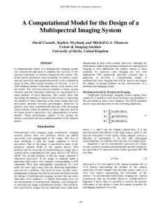
Fig. 1—Schematic phase equilibrium diagram of the multicomponent FeC-M system.

A. Thermodynamics Model A generic equilibrium phase diagram of the multicomponent Fe-C-M system is schematically shown in Figure 1, where M represents any combination of alloy element additions of Mn, Si, Ni, Cr, Mo, Cu, V, W, and Nb. In such a multicomponent system, peritectic and eutectoid reactions are no longer taking place at a constant temperature as in the binary Fe-C system, but within a temperature range. For the eutectoid reaction, the authors have designated Ae1 and As1 as the upper and lower limits of the eutectoid range in steel. Physically, Ae1 represents the asymptote of pearlite start curve in a time-temperature-transformation (TTT) diagram and As1 the asymptote of pearlite finish curve in a TTT diagram. Equilibrium temperature range for the peritectic reaction can be computed in a similar manner. The thermodynamic model developed in this study is able to compute equilibria in any low alloy steel system. However, it is only Ae3, Ae1, As1, and the eutectoid composition that are of concern in the modeling of a conventional heat treating process. Thus, only this part of the thermodynamic model is presented in this article. The thermodynamics model developed by the authors is based on the pioneering work of Kirkaldy and co-workers.[5–8] In their original work, the chemical potentials for each element were expressed using the Wagner[9] formulation. The following simplifying assumptions were made. (1) Carbon content in ferrite was negligible and the selfinteraction coefficient of carbon in ferrite was thus set to zero. 662—VOLUME 29B, JUNE 1998

Σε

i52

1i

Xi

[1]

n

m1 5 7G1 1 RT ln X1 1 RT bution in the Jominy bar. The reaction kinetics model predicts austenite decomposition reactions so that the resultant microstructure is predicted. Consequently, the Jominy hardness is calculated based on the microstructure. The predicted results were then compared and validated with experimental measurements.

Σε

n

1i

i51

Xi

[2]

mi 5 7Gi 1 RT ln Xi 1 RT (ε1i X1 1 εii Xi)

[3]

where 7Gi is the standard free energy of element i in infinite dilute iron solution; and Xi denotes the mole fraction of element i, εli the interaction coefficient between carbon and element i, and εii the self-interaction coefficient of element i. Note that the self-interactions of substitutional alloying elements have been introduced into the thermodynamics model, in Eqs. [1] and [3], by the εli term. The Gibbs free energy of carbides including cementite is described by the subregular solution model originally proposed by Richardson[11] and by Hillert and Staffensson.[12] This model is used in this research to model the g-cementite equilibrium. In the formulation of this model, all thermodynamic quantities are referred to one mole of metal atoms. The carbide formula M3C was thus rewritten as MC1/3. The chemical potentials of the carbides are expressed by mFeC1/3 5 mi 1

1 m 5 7GFeC1/3 1 RT ln Y0 1 3 1

mMC1/3 5 mi 1

ΣAY n

i52

0i

2 i

1 m 3 1

[4]

[5]

ΣA n

5 7GMC1/3 1 RT ln Yi 1

i52

0i

(1 2 Yi )2

In these two equations, Y0 and Yi (i 5 2 to n) are concentrations of metal elements in cementite expressed by Yi 5 Xi/(1 2 Xi) 5 4Xi/3 for i 5 0, 2 to n, which represents the fraction of lattice sites occupied by element i. The parameter A0i is the interaction coefficient between iron and substitutional alloying element i in the carbides. Interactions between substitutional alloying elements in carbides are justifiably neglected. Details of the model formulation, thermodynamics database, numerical schemes, and model validation are not METALLURGICAL AND MATERIALS TRANSACTIONS B

Fig. 2—Predicted Ae3 and measured AF temperatures.[14]

Fig. 3—Predicted As1 and measured As temperatures.[14]

Raphson method to the key variable, normally the temperature, and by using a simple iterative method for the other variables. For the computations of three-phase equilibria, the Newton–Raphson method was used for the two key variables, normally the ternary phase equilibrium temperature and the carbon content in one of the phases. Other variables were determined using simple iterative schemes. The accuracy and reliability of this thermodynamics model were validated with earlier reported experimental measurements. Computed phase transformation temperatures are presented in Figures 2 and 3 in comparison with the experimental measurements by Grange.[13] In Grange’s measurements, AS is called austenite start temperature, which represents the temperature at which a barely detectable amount of austenite forms during prolonged holding at constant temperature, and AF is the temperature at which the last trace of ferrite transforms to austenite on prolonged isothermal holding. Consequently, AS and AF correlate to the As1 and Ae3 in this thermodynamics model. Excellent agreement is observed between the computed and measured phase transformation temperatures. For the given data of 19 steels, the mean difference between computed Ae3 and measured AF temperatures is 21.5 7C, and the root-mean-square difference is 5.2 7C. The mean difference between computed As1 and measured AS temperatures is 27.8 7C, and the root-mean-square difference is only 8.5 7C. Computed equilibrium phase transformation temperatures provide the basis for latter calculation of undercooling for ferrite and pearlite reactions. They themselves are also useful in choosing proper heat treatment temperatures. A by-product of this thermodynamics model is the heat of solid-state phase transformations and the latent heat of fusion. Consequently, the enthalpy change of steel can be estimated. The predicted enthalpy changes of steel are found to be in excellent agreement with those published in handbooks.[14] B. Finite Element Heat Transfer Model

Fig. 4—Finite element model for the heat transfer analysis.

presented in this article. Interested readers are referred to Reference 13 for such information. For the computations of two-phase equilibria, one needs to solve a group of nonlinear equations. This was done by applying the Newton– METALLURGICAL AND MATERIALS TRANSACTIONS B

A two-dimensional axisymmetric finite element model was developed to analyze the heat transfer induced by end quenching of Jominy bars using the commercial code ANSYS. The finite element model is presented in Figure 4. The density of Jominy bars was assumed to remain constant at the room-temperature value, 7860 kg/mm3. Temperaturedependent thermal conductivity and enthalpy change of materials are readily available in the literature for many commercial steels.[14] The convective film coefficient at the quenching end was estimated from the working formulas for forced convection assuming a water jet passes a noncircular object.[15] The cylindrical and top surfaces of a Jominy bar are subject to free convection in air and radiation. Heat loss through these free surfaces was incorporated into the analysis by introducing the combined heat transfer coefficient that accounts for both convection and radiation. Normally, the surface heat transfer by convection, qc, is described by Newton’s law of cooling: qc 5 Ahc (Ts 2 Ta)

[6]

in which A is the surface area, hc is the convective heat transfer coefficient, Ts is the surface temperature, and Ta represents the ambient temperature. It is known that the VOLUME 29B, JUNE 1998—663

convective heat transfer coefficient, hc, is temperature dependent. The radiant heat transfer from a surface, qr, is represented by qr 5 Asε (T 4s 2 T 4a)

[7]

In Eq. [7], s is the Stefan–Boltzmann constant with the value of 56.7 W/mm. K and ε is the radiation emissivity of the surface. Quite often in numerical heat transfer analysis, Eq. [7] is linearized into the form qr 5 Ahr (Ts 2 Ta)

[8]

by the introduction of the radiation coefficient hr: hr 5 sε

(T 4s 2 T 4a) 5 sε (T s2 1 T a2)(Ts 1 Ta) (Ts 2 Ta)

[9]

It is apparent that the radiation coefficient, hr, is strongly dependent on the temperature. The use of the radiation coefficient allows one to express the combined heat flow from the surface as q 5 qc 1 qr 5 A(hc 1 hr)(Ts 2 Ta)

two models are similar but differ in details. Like the Kirkaldy model, the general form of TTT in this model is described by Zener[22] and Hillert[23] type formulas:

t (X,T ) 5

X

S(X) 5

0.4(12X )

C. Austenite Grain Size

dX DT n exp (2Q/RT) X 0.4(12X ) (1 2 X)0.4X 5 dt F(C,Mn,Si,Ni,Cr,Mo,G)

[11]

where a, b, and c are constants depending on whether the steel has grain growth modifiers. D. Reaction Kinetics Model for Austenite Decomposition The reaction kinetics model developed in this study is based on modifying the original model developed by Kirkaldy and Venugopalan.[3] The basic methodologies of these

[13]

[14]

Equation [14] can be used to calculate the reaction rate at any instant of time as a function of temperature, prior austenite grain size, steel composition, and volume fraction of transformed products. With the application of the additivity rule, Eq. [14] can be readily used to predict the amount of phase transformation under arbitrary cooling conditions by doing the integration along the temperature-time curve: X5

One important microstructural parameter in the prediction of steel hardenability is the austenite grain size. The authors have compiled a rather large collection of empirically based models for the prediction of prior austenite grain growth. In this study, for the prediction of Jominy hardness, the prediction of prior austenite grain size is quite simple. The authors have adopted the grain growth kinetics equation proposed by DeAndre´s and Carsı´:[21]

dX (1 2 X)0.4X

When X → 0, Eq. [13] predicts X } t1.67, which corresponds to the empirical observation t1.0 pct ' 4 3 t0.1 pct made by Kirkaldy et al.[6] Computing phase transformations under continuous cooling is straightforward with the application of the additivity rule. Equation [12] can be rewritten as

X

664—VOLUME 29B, JUNE 1998

*X 0

in which hcr 5 hc 1 hr is called the combined heat transfer coefficient. Note that Eq. [10] is in the same form as Newton’s law of cooling. Coefficients of free convection, hc, were calculated based on analytical working formulas for free convection presented by Churchill and Chu[16] and by Goldstein et al.[17] The commonly reported emissivity value, ε, of steel surfaces varies from less than 0.1 to around 0.8 depending upon surface finish, amount of oxidation, and temperature.[18,19,20] A constant emissivity value of 0.3 was used in this analysis. The temperature dependence of the combined heat transfer coefficient was calculated prior to the heat transfer analysis. In the numerical analysis, the calculated combined heat transfer coefficients were applied to free surfaces in the same manner as applying purely convection boundary conditions.

a 1 b ln t 1 c T

[12]

where F is a function of steel composition C, Mn, Si, Ni, Cr, and Mo in wt pct; and G is the prior austenite grain size (ASTM number), DT is the undercooling, and Q is the activation energy of the diffusional reaction. The exponent of undercooling n is an empirical constant determined by the effective diffusion mechanism (n 5 2 for volume and n 5 3 for boundary diffusion). S(X) is the reaction rate term, which is an approximation to the sigmoidal effect of phase transformations. The major differences in the formulation of the present model and the Kirkaldy model are the expression of F(C, Mn, Si, Ni, Cr, Mo, G) and the sigmoidal effect term S(X). The significance of these differences is discussed later in section V, part D. S(X) in this model is expressed in the form of

[10]

5 Ahcr (Ts 2 Ta)

G5

F(C,Mn,Si,Ni,Cr,Mo,G) S(X) DT n exp (2Q/RT)

t

* dX 5 * dXdt dt 0

0

t

5

* DT 0

n

exp (2Q/RT) X 0.4(12X ) (1 2 X)0.4X dt F(C,Mn,Si,Ni,Cr,Mo,G)

[15]

In a TTT diagram, the location of the ‘‘nose’’ of each C curve correlates to the maximum reaction rate. Note that the formulation of Eq. [12] suggests that the curvature of each C curve in a TTT diagram is primarily determined by the activation energy of the reaction. The exact locations of the nose are jointly determined by the values of n and Q. From Eq. [12], at the nose temperature, the author derived d (DT n exp (2Q/RT)) 5 0 dT

[16]

which leads to the relationship Q5

nRT 2N DT

[17]

METALLURGICAL AND MATERIALS TRANSACTIONS B

where TN is the temperature at the nose position. By calibrating Eq. [16] with published TTT diagrams,[24] one can get good estimations of the optimal value of Q. For the estimated data available, it was found that the Q values have a median value of 27,500 kcal/mol 7C. For simplicity of the reaction kinetics model, the authors have chosen to use this single value of Q. After determining the value of the activation energy, the authors proceeded to determine the kinetics coefficient of alloying elements in Eq. [12] by calibrating Eq. [14] with continuous cooling transformation (CCT) diagrams in the open literature. Eventually, the authors were able to develop a new set of kinetics equations to describe austenite decomposition reactions. Under isothermal conditions, the ferrite reaction can be represented by

tF 5

20.41G

FC S(X) (Ae3 2 T)3 exp (227,500/RT)

[18]

where the effects of alloying elements on the ferrite reaction are expressed by FC 5 exp (1.00 1 6.31C 1 1.78Mn 1 0.31Si 1 1.12Ni 1 2.70Cr 1 4.06Mo)

[19]

The pearlite reaction is represented by

tP 5

PC S(X) 20.32G (Ae1 2 T)3 exp (227,500/RT)

[20]

and the effects of alloying elements on the pearlite reaction are expressed by PC 5 exp (24.25 1 4.12C 1 4.36Mn 1 0.44Si

[21]

1 1.71Ni 1 3.33Cr 1 5.19=Mo) The bainite reaction under isothermal condition is represented by

tB 5

2

0.29G

BC S(X) (BS 2 T) exp (227,500/RT) 2

[22]

where the effects of alloying elements on the bainite reaction are expressed by BC 5 exp (210.23 1 10.18C 1 0.85Mn 1 0.55Ni 1 0.90Cr 1 0.36Mo)

[23]

The undercooling terms for ferrite and pearlite reactions can be readily calculated using the Ae3 and Ae1 temperatures computed from the thermodynamic model. To calculate the undercooling for bainite reaction, the present authors decided to use the asymptote of the bainite start curve in TTT diagrams. This methodology was also used in the Kirkaldy and Venugopalan model.[3] When compared with the data presented in the isothermal transformation diagrams in the U.S. Steel Atlas,[24] it was found that the original equation for estimating the bainite start temperature, Bs, in the Kirkaldy model overestimated the suppressing effect of Si. For most low alloy steels, Si content is kept around 0.25 pct. This poses no problem in using the Bs equation in the Kirkaldy model. The predicted Bs temperatures for steels with higher Si content, i.e., ;1.0 pct or above, are too low when compared with bainite asymptote temperatures in published TTT diagrams for Si containing steels.[24] Earlier work by Steven and Haynes[25] suggested that the effect of Si on Bs METALLURGICAL AND MATERIALS TRANSACTIONS B

temperature is negligible. So the authors modified Kirkaldy’s Bs equation by normalizing the coefficient of Si in Kirkaldy’s Bs temperature equation at Si 5 0.25 pct. The modified Bs equation is expressed by BS (7C) 5 637 2 58C 2 35Mn

[24]

2 15Ni 2 34Cr 2 41Mo The Ms formula proposed by Kung and Raymond[26] based on modification of the original linear formula by Andrews[27] was adopted in this model: MS (7C) 5 539 2 423C 2 30.4Mn 2 17.7Ni

[25]

2 12.1Cr 2 7.5Mo 1 10Co 2 7.5Si Kung and Raymond reported that this formula has better accuracy than the Ms formula of Steven and Haynes.[25] E. Hardness Calculation The hardness distribution along the Jominy bar was calculated using the rule of mixtures: Hn 5 XM HnM 1 XB HnB 1 (XF 1 XP)HnF1P

[26]

where Hv is the hardness in Vickers; XM, XB, XF, and XP are the volume fraction of martensite, bainite, ferrite, and pearlite, respectively; and HvM, HvB, HvF1P are the hardness of martensite, bainite, and the mixture of ferrite and pearlite, respectively. Empirically based formulas developed by Maynier et al.[28] were used in the study for the calculation of HvM, HvB, and HvF1P as functions of steel composition and cooling rate: HnM 5 127 1 949C 1 27Si 1 11Mn

[27]

1 8Ni 1 16Cr 1 21 log Vr HnB 5 2323 1 185C 1 330Si 1 153Mn 1 65Ni 1 144Cr 1 191Mo 1 (89 1 53C 2 55Si 2 22Mn 2 10Ni 2 20Cr 2 33Mo) log Vr

[28]

HnF1P 5 42 1 223C 1 53Si 1 30Mn 1 12.6Ni 1 7Cr 1 19Mo 1 (10 2 19Si 1 4Ni 1 8Cr 1 130V) log Vr

[29]

where Vr is the cooling rate at 700 7C in degrees Celsius per hour. III.

MATERIALS AND EXPERIMENT

When considering validation of the quantitative prediction of steel hardenability, it is natural to think about using the existing hardenability data sets for the model validation. However, it is important to recognize the inherent limitations of the existing Jominy hardness curves. The international resource of TTT, CCT diagrams, and Jominy hardness curves consists of some 1000 sets with highly varying quality.[29] Kirkaldy and Feldman[30] summarized the reported Jominy hardness curves by several laboratories on 4140 steel of approximately the same composition and VOLUME 29B, JUNE 1998—665

Table I.

Composition of Steels (Weight Percent)

Steel

C

Mn

Si

Ni

Cr

Mo

W

Cu

Al

V

A36 A588 4140 4340 Class 1

0.20 0.24 0.38 0.41 0.24

1.01 0.98 0.81 0.74 0.31

0.10 0.10 0.28 0.25 0.20

0.02 0.02 0.11 1.72 3.04

0.02 0.02 0.98 0.77 0.39

— — 0.22 0.27 0.44

0.002 0.001 0.003 0.007 0.011

0.05 0.04 0.11 0.07 0.09

0.005 — 0.051 0.027 0.001

0.002 0.001 0.003 0.002 0.052

Fig. 7—Predicted cooling rates at 700 7C along the Jominy bars.

IV.

RESULTS

A. Thermal Cycles in the Jominy Bar

Fig. 5—Comparison between the predicted and measured thermal cycles.[31]

Fig. 6—Computed thermal cycles for a point 1 in. away from the quenching end.

grain size. The reported discrepancy is so significant that it discouraged the authors from using these data sets without discretion. The authors thus decided to conduct their own experiment for the model validation as well as comparing the experimental measurements and model predictions with those presented in the open literature. Jominy end-quench tests were conducted for five selected steels with various hardenability. Steels selected include ASTM A36, ASTM A588, AISI 4140, AISI 4340, and MIL-S-23284 Class 1. The compositions of these steels are listed in Table I. The standard end-quench test procedure, ASTM A25589, was followed. Hardness measurements were normally done with Rockwell C. When hardness values became less than 20 HRC, however, hardness was measured in Vickers. 666—VOLUME 29B, JUNE 1998

Finite element analysis revealed that the cooling rates in different Jominy bars are virtually the same despite minor differences in austenization temperatures and thermal properties of steels. The predominant heat transfer mechanism in the end quench of Jominy bars is the forced convection at the quenching end. Heat is primarily carried away by the quenching water. Heat loss through free convection and radiation at the cylindrical and top surfaces of the Jominy bar is less significant. The predicted thermal cycles in the Jominy bars are found to be in good agreement with the experimentally measured results by Birtanlan et al.[31] (Figure 5). The results from finite element analysis were also compared with those from the analytical solution proposed by Kirkaldy et al.[3,6] All these solutions are found to be in good agreement with each other. They all suggest that the cooling rates in different Jominy bars are virtually identical despite the differences in steel composition, material properties, and austenization temperatures. Typical comparisons between the finite element solutions and the analytical solutions are presented in Figures 6 and 7. Computed thermal cycles at a point 1.0 in. (25.4 mm) away from the quenched end of an AISI 4140 steel Jominy bar are presented in Figure 5. The computed cooling rates at 700 7C along the Jominy bars are shown in Figure 6. When comparing the finite element solution in this study with the analytical solution by Kirkaldy et al., it should be noted that free convection and radiation at the cylindrical and top surfaces were ignored during the derivation of the analytical solution. It is interesting to note that the analytical solution agrees quite well with the finite element solution, with convection and radiation considered at short times. At longer times, the analytical solutions are found to be in better agreement with the finite element solution, without considering convection and radiation. B. Microstructure and Hardness For all the steel samples in this study, the estimated grain size G numbers using Eq. [11] were around 8. The predicted and measured hardness distributions along Jominy METALLURGICAL AND MATERIALS TRANSACTIONS B

Fig. 8—Predicted and measured Jominy hardnesses of ASTM A36 steel.

Fig. 11—Predicted and measured Jominy hardnesses of MIL-S-23284 Class 1 steel.

Fig. 9—Predicted and measured Jominy hardnesses of ASTM A588 steel.

Fig. 12—Predicted and measured Jominy hardnesses of AISI 4340 steel.

volume fractions in Jominy bars of five different steels are presented in Figure 13. V.

DISCUSSION

A. Cooling Rate in Jominy Bars

Fig. 10—Predicted and measured Jominy hardnesses of AISI 4140 steel.

bars are presented in Figures 8 through 12. Good agreement is observed between the measured and the predicted hardness values using this model. For the sake of comparison, predictions using the Kirkaldy model are also plotted. The present model has demonstrated considerable improvement over the original Kirkaldy model. The predicted martensite METALLURGICAL AND MATERIALS TRANSACTIONS B

Computational results in this study showed that changes of steel composition, material thermal properties, and austenization temperature have negligible effects on the cooling rate in Jominy bars. This is because changes related to these variables are rather minor. Comparison of the cooling rates in Jominy bars predicted with the finite element solutions and with the analytical solution developed by Kirkaldy revealed that they are in good agreement. The analytical solution has the advantage of simplicity. The finite element model, on the other hand, has more versatility and flexibility in incorporating complex geometry and boundary conditions. It is believed that the finite element solution presented in this article with the convection and radiation boundary conditions considered is a more realistic representation of the heat transfer in the actual Jominy bars. With the finite element solution, one can gage the error that might have been introduced into the analytical solution by ignoring the convective and radiative VOLUME 29B, JUNE 1998—667

purposes, the discrepancy can be ignored and the analytical solution can provide satisfactory solution for the prediction of Jominy hardness. For simple predictions such as Jominy hardness, the choice of one over the other would be totally up to the analyst and would depend on the specific objectives. The finite element model does have more advantages in analyzing the heat transfer induced by the heat treating of components with more complex geometry. B. Prediction of Phase Transformation Diagrams

Fig. 13—Predicted microstructure in Jominy bars.

Fig. 14—Comparison between the predicted and measured TTT diagrams for a 4140 steel:[25] C 5 0.37, Mn 5 0.77, Si 5 0.15, Ni 5 0.04, Cr 5 0.98, Mo 5 0.21, and G 5 7 to 8. Transformation start: 0.1 pct; and transformation finish: 99.9 pct.

The present model, as well as the Kirkaldy model, was formulated in Zener–Hillert type kinetics equations. Both models can be readily used to predict TTT diagrams. They can also be implemented to predict CCT diagrams provided the cooling conditions are known. The predicted TTT diagram using the present model for a typical alloy steel, AISI 4140, is presented in Figure 14 in comparison with the experimentally determined TTT diagram in the U.S. Steel Atlas.[24] The reported chemical composition and prior austenite grain size in the literature were used in the calculation. The predicted TTT diagram using the present model is in reasonably good agreement with the experimentally determined diagram, particularly in light of the problems associated with empirical transformation definition techniques used, as mentioned later. The original Kirkaldy model’s predictions for this alloy are similar to the authors’ model predictions and also agree reasonably well with the experimental data.[24] Note that the curves representing the start of phase transformations in the U.S. Steel Atlas are associated with the time for the formation of 0.1 pct of the transformed products. A predicted CCT diagram for the 4140 steel with the same composition for the prediction of the TTT diagram in Figure 14 is presented in Figure 15. Note that the C curve representing the start of a phase transformation in this predicted CCT diagram is associated with the formation of 1.0 pct volume fraction of the transformation product. The time scale starts at cooling from the Ae3 temperature. The predicted CCT diagram is in good agreement with those reported in the open literature.[32–35] C. Prediction of Steel Hardenability A practical indication of steel hardenability is the critical minimum cooling rate for the formation of a fully martensitic microstructure. In this study, it was assumed that this critical minimum cooling rate can be determined by the larger of the rates for the formation of 1.0 pct ferrite or 1.0 pct bainite. From the reaction kinetics model, the cooling rate for the formation of 1.0 pct ferrite under continuous cooling can be calculated from BS

V1.0

pct F

5

* t dT Ae3

Fig. 15—Predicted CCT diagrams of a 4140 steel: C 5 0.37, Mn 5 0.77, Si 5 0.15, Ni 5 0.04, Cr 5 0.98, Mo 5 0.21, G 5 7 to 8. Transformation start: 1.0 pct; and transformation finish: 99.9 pct.

heat loss at free surfaces. As one can see, this study demonstrated that the potential error is very small. For practical 668—VOLUME 29B, JUNE 1998

1.0 pct F

BS

5

* Ae3

Q (Ae3 2 T )3 exp (2 ) dT RT FC z S(X )X50.01

[30]

The cooling rate for the formation of 1.0 pct bainite under continuous cooling can be estimated using a similar equation. The Kirkaldy model can also be formulated in such a way to predict such cooling rates. Assuming linear cooling (constant cooling rates), the predicted critical minimum cooling rates for the formation of a fully martensitic miMETALLURGICAL AND MATERIALS TRANSACTIONS B

Table II.

Predicted Minimum Cooling Rates (Degrees Celsius Per Second) for the Formation of Fully Martensitic Structure

Model

ASTM A36

Present model Kirkaldy[3] DeAndre´s–Carsı´[21] Maynier et al.[36]

759 (F) 236 (B) 747 (B) 402 (B)

ASTM A588 515 210 515 283

(B) (B) (B) (B)

AISI 4140

MIL-S-23284 Class 1

AISI 4340

24.8 (B) 29.4 (F) 24.1 (B) 27.6 (B)

28 (B) 23 (F) 27 (B) 12 (B)

6.4 (B) 17 (F) 6.4 (B) 4.1 (B)

Note: The B and F in parentheses are the first nonmartensitic microstructure constituents, which represent the phase transformation that determines steel hardenability.

Table III. Predicted Cooling Rates (Degrees Celsius per Second) for the Formation of 50 Pct Ferrite Model

AISI 4140

MIL-S-23284 Class 1

AISI 4340*

Present model Kirkaldy[3] DeAndre´s–Carsı´[21] Maynier et al.[36]

0.67 6.34 1.15 0.97

0.16 5.91 0.03 0.07

0.11 3.11 0.09 0.14

*The computed equilibrium amount of ferrite in this steel is 39 pct. Thus, the predicted cooling rates in this column are for the maximum cooling rate for the ferrite reaction to reach completion.

crostructure as well as the phases that determine the critical minimum cooling rate for the five steels in this study are presented in Table II. These data are presented for the present model and the Kirkaldy model along with predictions using other methods that are based on empirical representations of CCT diagrams.[21,36] The predicted critical minimum cooling rates and martensite limiting phase products using the present model are in good to excellent agreement with those predicted using the model by Maynier et al.[36] and that by DeAndre´s and Carsı´,[21] respectively. The critical minimum cooling rate predictions given by the Kirkaldy model are in fair agreement with those predicted using the empirical methods, but differ in the predicted nonmartensitic microstructure that determines the steel hardenability. Thus, even through the Kirkaldy model gives reasonable predictions for the critical minimum cooling rates, it incorrectly predicts the martensite limiting phase. Both the present model and the Kirkaldy model were formulated to calculate the critical cooling rate for the formation of 50 pct ferrite. The predicted results for the three hardenable steels were compared with the predictions using empirical methods.[21,36] The comparison is shown in Table III. Note that for AISI 4340 steel, since the predicted equilibrium amount of ferrite is 39 pct, the maximum cooling rate for the ferrite reaction to reach completion is presented instead. For the three hardenable steels, the predictions given by the present model are in good agreement with those given by the empirical models. The predicted cooling rates for the formation of 50 pct ferrite in these three steels using the Kirkaldy model are significantly higher than those predicted using empirical methods. It is not surprising that both the present model and the Kirkaldy model came up with predictions in Table II that are in reasonable agreement with those predicted with empirical methods. This is because both the models were calibrated with the phase transformation start curves, the present model with CCT diagrams and the Kirkaldy model with TTT diagrams. There exists a significant difference METALLURGICAL AND MATERIALS TRANSACTIONS B

between the predicted first nonmartensitic microstructures predicted with the present model and those predicted with the Kirkaldy model. The Kirkaldy model predicts that the minimum cooling rates for the formation of fully martensitic microstructure are determined by the ferrite reaction in three hardenable steels, AISI 4140, MIL-S-23284 Class 1, and AISI 4340, whereas the present model predicts that the first nonmartensitic microstructure in these steels is bainitic. The comparison shown in Table II reveals that the Kirkaldy model tends to underestimate the incubation time of the ferrite reaction. The comparison shown in Table III further demonstrates that the Kirkaldy model overestimates the rate of ferrite reaction by a significant factor. It is believed that these are the two major reasons why the Kirkaldy model underestimates the hardenability of steels with medium and high concentrations of alloying elements. D. Differences between the Present Model and the Kirkaldy Model The present model was developed based on reconstituting the original Kirkaldy model[3] with a different philosophy in model formulation and calibration. These modifications are considered imperative to making realistic predictions. The following discussion is focused on the insights into and implications of model construction with special emphasis on the factors affecting steel hardenability. 1. Reaction rate: S(X) vs I(X) Both the present model and the Kirkaldy model were calibrated with phase transformation start curves: t0.1 pct in TTT diagrams for the Kirkaldy model, and critical cooling rate for the formation of 1.0 pct phase transformation product in CCT diagrams for the present model. Assuming they all predict the incubation time for a reaction with reasonable accuracy, the reaction rate would be dependent on the S(X) and I(X) terms for the present model and the Kirkaldy model, respectively. For the ferrite and pearlite reactions, it is interesting to note the ratio between the time to finish and the time to start the reaction (X ' 1.0 pct). The Kirkaldy model used the I(X) expression, X

I(X) 5

*X 0

2(12X )/3

dX (1 2 X)2X /3

[31]

to simulate the sigmoidal effect of phase transformations. This expression would predict I(1.0)/I(0.01) 5 7.2, i.e., tFf/tFs 5 7.2 at any temperature. In addition, the formulation of the I(X) term in Eq. [31] would yield t(1.0 pct)/t(0.1 pct) VOLUME 29B, JUNE 1998—669

5 2.15, which contradicts the empirical observation by Kirkaldy of t(1.0 pct)/t(0.1 pct) ' 4.[6] The I(X) term in the Kirkaldy model was replaced with an S(X) term in the present model. The S(X) term (Eq. [13]) would predict t(1.0 pct)/t(0.1 pct) ' 4 and X } t1.7 in the early stage of phase transformation, which is consistent with the empirical observation by Kirkaldy et al.[6] After making this change, the present model would predict S(1.0)/S(0.01) 5 19.9, i.e., tFf /tFs 5 19.9. The characteristics of S(X) and I(X) terms are shown in Figure 16. Note that the difference in the formulation of S(X) and I(X) terms indicates that the predicted reaction rate in the Kirkaldy model is approximately 3 times faster than that predicted with the present model. Given the fact that both the present model and the Kirkaldy model predicted TTT diagrams of AISI 4140 steel with comparable agreement with the experimental TTT diagram in the U.S. Steel Atlas, it is interesting to note that the predicted Jominy hardness curves differ by a significant factor (Figure 10). The comparison between I(X) and S(X) terms offers an explanation, in the perspective of reaction rate, why the Kirkaldy model underestimates the hardenability for steels with medium and high alloying element contents. In this study, it was not necessary to incorporate another empirical term to simulate the sluggishness of bainite reactions, as was done in the Kirkaldy model. This indicates that the reaction rate discrepancies introduced by the I(X) term in the Kirkaldy model forced the use of a supplemental correction term in their I'(X) expression for the prediction of bainite reaction. 2. Effects of alloying elements: additive vs multiplicative All empirically based models[1,2,21,36] suggest that the effects of alloying elements on steel hardenability are multiplicative. The Kirkaldy model, however, implies that they are additive, which contradicts experimental observations. This was introduced by their approximation of the effective diffusion coefficient of phase transformation: 1 1 5 1 Deff Dc

Σ kDC n

i

i52

i

[32]

i

In theory, the effects of alloying elements on steel hardenability are twofold: thermodynamic and kinetic. Thermodynamically, they affect steel hardenability by influencing the equilibria of the Fe-C-M multicomponent system. Thus, they either enlarge or suppress the temperature region for each austenite decomposition reaction. The kinetic effects of alloying elements on steel hardenability are that they all retard austenite decomposition reactions through partitioning at the phase boundaries. Essentially, all alloying elements increase steel hardenability in different degrees. The present model was formulated in such a way that the kinetic effects of alloying elements are multiplicative, which reflects experimental observations. Sensitivity studies with the current model showed that the kinetic effects of alloying elements on steel hardenability are more pronounced than their thermodynamic effects. When the concentration of alloying elements is small, it does not make much difference, from a mathematical point of view, whether the effects of alloying elements are additive or multiplicative. The difference, however, will become more pronounced as the alloying element content in670—VOLUME 29B, JUNE 1998

Fig. 16—Characteristics of I(X) and S(X) terms.

creases. The formulation of the effective diffusion coefficient in the Kirkaldy model explains why it works reasonably well for less hardenable steels, but significantly underestimates steel hardenability for steels with medium and high concentrations of alloying elements. Carbon content was not explicitly present in Kirkaldy’s kinetics equations. This implies that the effect of carbon content on steel hardenability is only through its thermodynamic effects on the Ae3, Ae1, Bs, and Ms temperatures. Experimental studies in the open literature revealed that carbon content has a significant effect on steel hardenability. The coefficients for carbon content in the kinetic equations of the present model, Eqs. [19], [21], and [23], clearly indicate that the carbon content in the steel is probably the most significant factor in determining steel hardenability. 3. Database for the model calibration: TTT diagrams vs CCT diagrams Both the present model and the Kirkaldy model predict TTT diagrams with reasonable agreement with the experimentally determined TTT diagrams presented in the open literature. But the predicted microstructures in the Jominy bars are significantly different from each other for hardenable steels. Results obtained from this study suggest that being able to predict TTT diagrams with reasonable accuracy does not necessarily mean that the model can give good predictions for the phase transformations under continuous cooling conditions. There are two limitations in using the TTT diagrams in the U.S. Steel Atlas[24] for the prediction of phase transformations under continuous cooling conditions. First, those TTT diagrams in the U.S. Steel Atlas had a lot of uncertainties in the precision of determining phase transformation start times. The Appendix of the U.S. Steel Atlas states that the exact location of the curves on the time scale, which represent the start of phase transformations, designated as the formation of 0.1 pct volume fraction of transformed product, is not highly precise, particularly for those reaction times less than 2 seconds. In reality, this quantity of transformed product is barely detectable by metallographic examination. The C curves in the U.S. Steel Atlas[24] were estimated from longer reaction times when substantial amounts of phase transformation products had formed. The estimation was based on the kinetics theory originally proMETALLURGICAL AND MATERIALS TRANSACTIONS B

posed by Austin and Rickett.[37] Second, the majority of TTT diagrams in this compendium do not have discrete ferrite and bainite noses but a common nose temperature for the combined ferrite and bainite reactions. Thus, calibration of the ferrite and bainite reaction initiation times based on the data presented in this compendium was difficult, if not impossible. The CCT diagrams, on the other hand, are measured under more realistic and most likely more measurable cooling conditions for the determination of phase transformation start curves. The majority of CCT diagrams in the open literature were obtained using a dilatometry method followed by metallographic examinations, and they exhibit discrete ferrite and bainite noses. This was the reason that the authors decided to calibrate the present model with CCT diagrams. Thus, it is not surprising that the present model gives more accurate predictions to Jominy hardness than the Kirkaldy model for phase transformations under continuous cooling conditions. 4. Austenite grain size Originally, the Kirkaldy model had a grain size term 1/2(G21)/2, which literally represents the number of grains per square inch at magnification 100 times. A difference of 2 in ASTM grain size number G will affect steel hardenability by a factor of 2. This term has been recently adjusted by Kirkaldy[38] to 1/2G/8, which represents the 1/4 power of the austenite grain diameter D (D } 1/2G/2). A difference of 2 in austenite grain size number thus affects steel hardenability by a factor of 1.18. The rationale behind this adjustment was to match the incubation time transient predicted by Cahn[39] for nucleation and growth from grain boundaries. Classical phase transformation kinetics theory developed by Johnson and Mehl[40] and Avrami,[41] and perfected by Cahn,[39] is more complicated. Cahn[39] studied four types of nucleation sites: homogeneous nucleation, grain boundaries, grain boundary edges, and grain boundary corners. He analyzed the half time of a reaction and its dependence on the austenite grain diameter D. He concluded that the half time of a reaction is proportional to the D1/4 for grain boundary nucleation, D1/2 for edge nucleation, D3/4 for corner nucleation, D1 for site saturation, and D0 for homogeneous nucleation. It is the authors’ perception that all these nucleation sites are competing with each other during any phase transformation. The overall effect of the grain size on a reaction may be some kind of statistical average among all these nucleation mechanisms. The coefficient of grain size term in the present model may be interpreted as the overall effect of grain size. The coefficients of grain size in Eqs. [18], [20], and [22] reveal that the nucleation mechanism in ferrite reaction is close to site saturation, whereas grain boundary edges and corners are the dominating nucleation sites for pearlite and bainite reactions. From Eqs. [18], [20], and [22], one can expect that the ferrite reaction is more sensitive to prior austenite grain size than pearlite and bainite reactions. VI.

CONCLUSIONS

A fundamentally based and empirically calibrated model for austenite decomposition reactions has been presented in this article. Application of the present model in the predicMETALLURGICAL AND MATERIALS TRANSACTIONS B

tion of Jominy hardness of steels has demonstrated significant improvement of accuracy over the original Kirkaldy model. The effects of austenite grain size, alloy elements, and transformation kinetics parameters on steel hardenability have been discussed and readily accounted for in the present model. Incorporated with a proper heat transfer model, the models presented in this article for the prediction of microstructure and hardness can be used for the prediction of hardness in practical processes such as heat treating and welding.

ACKNOWLEDGMENTS The authors are grateful to Professor John Kirkaldy, McMaster University, and Professor Devarajan Venugopalan, University of Wisconsin, for the insightful discussions on the Kirkaldy model. Special thanks are due to Dr. Thompson Groeneveld, Battelle Memorial Institute (Columbus, OH), for his support and critique on the usage of terms in this manuscript. The authors also thank the editors and reviewers for the speed of the review and their comments, which strengthened the article.

REFERENCES 1. M.V. Li, D. Niebuhr, D.G. Atteridge, and L. Meekisho: Phase Transformations during the Thermal/Mechanical Processing of Steel, E.B. Hawbolt and S. Yue, eds., CIM, Montreal, 1995, pp. 485-501. 2. M. Li: Ph.D. Thesis, Oregon Graduate Institute of Science and Technology, Portland, OR, 1996. 3. J.S. Kirkaldy and D. Venugopalan: Phase Transformations in Ferrous Alloys, D.A.R. Marder and J.I. Goldstein, eds., AIME, New York, NY, 1983, pp. 128-48. 4. J.L. Lee and H.K.D.H. Bhadeshia: China Steel Technical Report No. 7, China Steel Corporation, Hsiao Kang, Kaohsiung, Taiwan, 1993, pp. 16-25. 5. J.S. Kirkaldy and E.A. Baganis: Metall. Trans. A, 1978, vol. 9A, pp. 495-501. 6. J.S. Kirkaldy, B.A. Thomson, and E.A. Baganis: Hardenability Concepts with Applications to Steel, D.V. Doane and J.S. Kirkaldy, eds., AIME, New York, NY, 1977, pp. 82-125. 7. K. Hashiguchi, J.S. Kirkaldy, T. Fukuzumi, and V. Pavaska: CALPHAD, 1984, vol. 8 (2), pp. 173-86. 8. A. Kroupa and J.S. Kirkaldy: J. Phase Equilibria, 1993, vol. 14 (2), pp. 150-61. 9. C. Wagner: Thermodynamics of Alloys, Addison-Wesley Publishing Co., Reading, MA, 1952. 10. B. Uhrenius: Hardenability Concepts with Applications to Steel, D.V. Doane and J.S. Kirkaldy, eds., AIME, New York, NY, 1977, pp. 2881. 11. F.D. Richardson: J. Iron Steel Inst., 1953, vol. 175, pp. 33-51. 12. M. Hillert and L.I. Staffansson: Acta Chem. Scand., 1970, vol. 24 (10), pp. 3618-26. 13. R.A. Grange: Met. Progr., 1961, vol. 70 (4), pp. 73-75. 14. The British Iron and Steel Research Association: Physical Constants of Some Commercial Steels at Elevated Temperatures, Butterworth and Co., London, 1953. 15. A.J. Chapman: Fundamentals of Heat Transfer, Macmillan Publishing Company, New York, NY, 1987. 16. S.W. Churchill and H.H.S. Chu: Int. J. Heat Mass Transfer, 1975, vol. 18, pp. 1323-29. 17. R.J. Goldstein, E.M. Sparrow, and D.C. Jones: Int. J. Heat Mass Transfer, 1973, vol. 16, pp. 1025-34. 18. F.P. Incropera and D.P. DeWitt: Fundamentals of Heat and Mass Transfer, John Wiley & Sons, New York, NY, 1985. 19. Smithells Metals Reference Book, 7th ed., E.A. Brandes and G.B. Brook, eds., Butterworths-Heinemann, London, 1992. 20. A.J. Chapman: Fundamentals of Heat Transfer, Macmillan Publishing Co., New York, NY, 1987. VOLUME 29B, JUNE 1998—671

21. M.P. DeAndre´s and M. Carsı´: J. Mater. Sci., 1987, vol. 22, pp. 270716. 22. C. Zener: Trans. AIME, 1946, vol. 167, pp. 550-83. 23. M. Hillert: Jernkont. Ann., 1957, vol. 141, pp. 557-85. 24. Atlas of Isothermal Transformation Diagrams, 3rd ed., U.S. Steel, Inc., Pittsburgh, PA, 1963. 25. W. Steven and A.G. Haynes: J. Iron Steel Inst., 1956, vol. 183, pp. 349-59. 26. C.Y. Kung and J.J. Rayment: Metall. Trans. A, 1982, vol. 13A, pp. 328-31. 27. K.W. Andrews: J. Iron Steel Inst., 1969, vol. 203, pp. 721-27. 28. P. Maynier, J. Dollet, and P. Bastien: Hardenability Concepts with Applications to Steels, D.V. Doane and J.S. Kirkaldy, eds., AIME, New York, NY, 1978, pp. 518-44. 29. Atlas of Time-Temperature Diagrams for Irons and Steels, G.F. Vander Voort, ed., ASM INTERNATIONAL, Materials Park, OH, 1991. 30. J.S. Kirkaldy and S.E. Feldman: J. Heat Treatment, 1989, vol. 1, pp. 57-64. 31. J. Birtanlan, R.G. Henley, Jr., and A.L. Christenson: Trans. ASM, 1954, vol. 46, pp. 927-47.

672—VOLUME 29B, JUNE 1998

32. Atlas of Isothermal Transformation Diagram, ASM, Metals Park, OH, 1977. 33. M. Atkin: Atlas of Continuous Cooling Transformation Diagrams for Engineering Steels, British Steel, Sheffield, England, 1977. 34. W.W. Cias: Phase Transformation Kinetics and Hardenability of Medium-Carbon Alloy Steels, Climax Molybdenum Company, Greenwich, CT, 1972. 35. W.W. Cias: Phase Transformation Kinetics of Selected Wrought Constructional Steels, Climax Molybdenum Company, Greenwich, CT, 1977. 36. P. Maynier, J. Dollet, and P. Bastien: Hardenability Concepts with Applications to Steels, D.V. Doane and J.S. Kirkaldy, eds., AIME, New York, NY, 1978, pp. 163-76. 37. J.B. Austin and R.L. Rickett: Trans. AIME, 1939, vol. 135, pp. 396415. 38. J.S. Kirkaldy: Scand. J. Metall., 1991, vol. 20, pp. 50-61. 39. J.W. Cahn: Acta Metall., 1956, vol. 4, pp. 449-59. 40. W.A. Johnson and R.F. Mehl: Trans. AIME, 1939, vol. 135, pp. 41642. 41. M. Avrami: J. Chem. Phys., 1939, vol. 7, pp. 1103-12.

METALLURGICAL AND MATERIALS TRANSACTIONS B