A COMPUTATIONAL THEORY OF DECISION ... - CiteSeerX

A COMPUTATIONAL THEORY OF DECISION NETWORKS By Nevin Lianwen Zhang B. Sc. (Mathematics) China University of Elect. Sci. & Tech. M. Sc., Ph. D. (Mathematics) Beijing Normal University a thesis submitted in partial fulfillment of the requirements for the degree of Doctor of Philosophy

in the faculty of graduate studies computer science We accept this thesis as conforming to the required standard

...................................................... ...................................................... ...................................................... ...................................................... ......................................................

the university of british columbia December 1993 c Nevin Lianwen Zhang, 1994

In presenting this thesis in partial fulfillment of the requirements for an advanced degree at the University of British Columbia, I agree that the Library shall make it freely available for reference and study. I further agree that permission for extensive copying of this thesis for scholarly purposes may be granted by the head of my department or by his or her representatives. It is understood that copying or publication of this thesis for financial gain shall not be allowed without my written permission.

Computer Science The University of British Columbia 2075 Wesbrook Place Vancouver, Canada V6T 1Z1

Date:

Abstract

This thesis is about how to represent and solve decision problems in Bayesian decision theory (e.g. Fishburn 1988). A general representation named decision networks is proposed based on influence diagrams (Howard and Matheson 1984). This new representation incorporates the idea, from Markov decision processes (e.g. Puterman 1990, Denardo 1982), that a decision may be conditionally independent of certain pieces of available information. It also allows multiple cooperative agents and facilitates the exploitation of separability in the utility function. Decision networks inherit the advantages of both influence diagrams and Markov decision processes. Both influence diagrams and finite stage Markov decision processes are stepwisesolvable, in the sense that they can be evaluated by considering one decision at a time. However, the evaluation of a decision network requires, in general, simultaneous consideration of all the decisions. The theme of this thesis is to seek the weakest graph-theoretic condition under which decision networks are guaranteed to be stepwise-solvable, and to seek the best algorithms for evaluating stepwise-solvable decision networks. A concept of decomposability is introduced for decision networks and it is shown that when a decision network is decomposable, a divide and conquer strategy can be utilized to aid its evaluation. In particular, when a decision network is stepwise-decomposable it can be evaluated not only by considering one decision at a time, but also by considering one portion of the network at a time. It is also shown that stepwise-decomposability is the weakest graphical condition that guarantees stepwise-solvability. Given a decision network, there are often nodes and arcs that can harmlessly removed. An algorithm is presented that is able to find and prune all graphically identifiable ii

removable nodes and arcs. Finally, the relationship between stepwise-decomposable decision networks (SDDN’s) and Markov decision process is investigated, which results in a two-stage approach for evaluating SDDN’s. This approach enables one to make use of the asymmetric nature of decision problems, facilitates parallel computation, and gives rises to an incremental way of computing the value of perfect information.

iii

Table of Contents

Abstract

ii

List of Figures

ix

List of symbols

xi

1 Introduction

1

1.1

Synopsis . . . . . . . . . . . . . . . . . . . . . . . . . . . . . . . . . . . .

2

1.2

Bayesian decision theory . . . . . . . . . . . . . . . . . . . . . . . . . . .

6

1.3

Decision analysis . . . . . . . . . . . . . . . . . . . . . . . . . . . . . . .

7

1.3.1

Decision trees . . . . . . . . . . . . . . . . . . . . . . . . . . . . .

8

1.3.2

Influence diagrams . . . . . . . . . . . . . . . . . . . . . . . . . .

11

1.3.3

Representing independencies for random nodes . . . . . . . . . . .

12

1.4

Constraints on influence diagrams . . . . . . . . . . . . . . . . . . . . . .

13

1.5

Lifting constraints: Reasons pertaining to decision analysis . . . . . . . .

15

1.5.1

Lifting the no-forgetting constraint . . . . . . . . . . . . . . . . .

15

1.5.2

Lifting the single value node constraint . . . . . . . . . . . . . . .

18

1.5.3

Lifting the regularity constraint . . . . . . . . . . . . . . . . . . .

19

Lifting constraints: Reasons pertaining to MDP’s . . . . . . . . . . . . .

21

1.6.1

Finite stage MDP’s . . . . . . . . . . . . . . . . . . . . . . . . . .

22

1.6.2

Representing finite stage MDP’s . . . . . . . . . . . . . . . . . . .

23

1.6

1.7

Computational merits

. . . . . . . . . . . . . . . . . . . . . . . . . . . .

25

1.8

Why not lifted earlier . . . . . . . . . . . . . . . . . . . . . . . . . . . . .

25

iv

1.9

Subclasses of decision networks . . . . . . . . . . . . . . . . . . . . . . .

26

1.10 Who would be interested and why . . . . . . . . . . . . . . . . . . . . . .

28

2 Decision networks: the concept 2.1

30

Decision networks intuitively . . . . . . . . . . . . . . . . . . . . . . . . .

30

2.1.1

33

A note . . . . . . . . . . . . . . . . . . . . . . . . . . . . . . . . .

2.2

Bayesian networks

. . . . . . . . . . . . . . . . . . . . . . . . . . . . . .

34

2.3

Decision networks . . . . . . . . . . . . . . . . . . . . . . . . . . . . . . .

36

2.3.1

A general setup of Bayesian decision theory . . . . . . . . . . . .

36

2.3.2

Multiple-decision problems . . . . . . . . . . . . . . . . . . . . . .

37

2.3.3

Technical preparations . . . . . . . . . . . . . . . . . . . . . . . .

38

2.3.4

Deriving the concept of decision networks

. . . . . . . . . . . . .

39

2.3.5

An example . . . . . . . . . . . . . . . . . . . . . . . . . . . . . .

41

Fundamental constraints . . . . . . . . . . . . . . . . . . . . . . . . . . .

42

2.4

3 Decision networks: formal definitions

45

3.1

Formal definition of Bayesian networks . . . . . . . . . . . . . . . . . . .

45

3.2

Variables irrelevant to a query

. . . . . . . . . . . . . . . . . . . . . . .

48

3.3

Formal definitions of decision networks . . . . . . . . . . . . . . . . . . .

50

3.4

A naive algorithm . . . . . . . . . . . . . . . . . . . . . . . . . . . . . . .

53

3.5

Stepwise-solvability . . . . . . . . . . . . . . . . . . . . . . . . . . . . . .

57

3.6

Semi-decision networks . . . . . . . . . . . . . . . . . . . . . . . . . . . .

59

4 Divide and conquer in decision networks

62

4.1

Separation and independence . . . . . . . . . . . . . . . . . . . . . . . .

63

4.2

Decomposability of decision networks . . . . . . . . . . . . . . . . . . . .

65

4.2.1

66

Properties of upstream and downstream components . . . . . . .

v

4.3

Divide and conquer . . . . . . . . . . . . . . . . . . . . . . . . . . . . . .

5 Stepwise-decomposable decision networks 5.1

69 71

Definition . . . . . . . . . . . . . . . . . . . . . . . . . . . . . . . . . . .

72

5.1.1

Another way of recursion . . . . . . . . . . . . . . . . . . . . . . .

74

5.2

Stepwise-decomposability and stepwise-solvability . . . . . . . . . . . . .

75

5.3

Testing stepwise-decomposability . . . . . . . . . . . . . . . . . . . . . .

76

5.4

Recursive tail cutting . . . . . . . . . . . . . . . . . . . . . . . . . . . . .

78

5.4.1

Simple semi-decision networks . . . . . . . . . . . . . . . . . . . .

79

5.4.2

Proofs . . . . . . . . . . . . . . . . . . . . . . . . . . . . . . . . .

80

5.5

Evaluating simple semi-decision networks . . . . . . . . . . . . . . . . . .

82

5.6

The procedure EVALUATE . . . . . . . . . . . . . . . . . . . . . . . . .

85

6 Non-Smooth SDDN’s 6.1

6.2

6.3

87

Smoothing non-smooth SDDN’s . . . . . . . . . . . . . . . . . . . . . . .

87

6.1.1

Equivalence between decision networks . . . . . . . . . . . . . . .

88

6.1.2

Arc reversal . . . . . . . . . . . . . . . . . . . . . . . . . . . . . .

88

6.1.3

Disturbance nodes, disturbance arcs, and disturbance recipients .

90

6.1.4

Tail-smoothing skeletons . . . . . . . . . . . . . . . . . . . . . . .

92

6.1.5

Tail smoothing decision networks . . . . . . . . . . . . . . . . . .

94

6.1.6

Smoothing non-smooth SDDN’s . . . . . . . . . . . . . . . . . . .

95

6.1.7

Proofs . . . . . . . . . . . . . . . . . . . . . . . . . . . . . . . . .

97

Tail and body . . . . . . . . . . . . . . . . . . . . . . . . . . . . . . . . .

99

6.2.1

Tail and body at the level of skeleton . . . . . . . . . . . . . . . . 100

6.2.2

Tail of decision networks . . . . . . . . . . . . . . . . . . . . . . . 101

6.2.3

Body of decision networks . . . . . . . . . . . . . . . . . . . . . . 103

The procedure EVALUATE1 . . . . . . . . . . . . . . . . . . . . . . . . . 105 vi

7

6.4

Correctness of EVALUATE1 . . . . . . . . . . . . . . . . . . . . . . . . . 107

6.5

Comparison to other approaches . . . . . . . . . . . . . . . . . . . . . . . 109 6.5.1

Desirable properties of evaluation algorithms . . . . . . . . . . . . 109

6.5.2

Other approaches . . . . . . . . . . . . . . . . . . . . . . . . . . . 112

Removable arcs and independence for decision nodes

118

7.1

Removable arcs and conditional independencies for decision nodes . . . . 119

7.2

Lonely arcs . . . . . . . . . . . . . . . . . . . . . . . . . . . . . . . . . . 121

7.3

Pruning lonely arcs and stepwise-solvability . . . . . . . . . . . . . . . . 123

7.4

Potential lonely arcs and barren nodes . . . . . . . . . . . . . . . . . . . 124

7.5

An algorithm . . . . . . . . . . . . . . . . . . . . . . . . . . . . . . . . . 125

8 Stepwise-solvability and stepwise-decomposability

127

8.1

Normal decision network skeletons . . . . . . . . . . . . . . . . . . . . . . 128

8.2

Short-cutting . . . . . . . . . . . . . . . . . . . . . . . . . . . . . . . . . 130

8.3

Root random node removal . . . . . . . . . . . . . . . . . . . . . . . . . . 135

8.4

Arc reversal . . . . . . . . . . . . . . . . . . . . . . . . . . . . . . . . . . 138

8.5

Induction on the number of random nodes . . . . . . . . . . . . . . . . . 142

8.6

Induction on the number of decision nodes . . . . . . . . . . . . . . . . . 145 8.6.1

An extension and a corollary . . . . . . . . . . . . . . . . . . . . . 147

8.7

Lonely arcs and removable arcs . . . . . . . . . . . . . . . . . . . . . . . 148

8.8

Stepwise-solvability and stepwise-decomposability . . . . . . . . . . . . . 150

9 SDDN’s and Markov decision processes 9.1

157

Sections in smooth regular SDDN’s . . . . . . . . . . . . . . . . . . . . . 158 9.1.1

An abstract view of a regular smooth SDDN . . . . . . . . . . . . 160

9.1.2

Conditional probabilities in a section . . . . . . . . . . . . . . . . 161

vii

9.2

9.1.3

The local value function of a section . . . . . . . . . . . . . . . . 161

9.1.4

Comparison with decision windows . . . . . . . . . . . . . . . . . 162

Condensing smooth regular SDDN’s . . . . . . . . . . . . . . . . . . . . . 163 9.2.1

Parallel computations . . . . . . . . . . . . . . . . . . . . . . . . . 165

9.3

Equivalence between SDDN’s and their condensations . . . . . . . . . . . 166

9.4

Condensing SDDN’s in general . . . . . . . . . . . . . . . . . . . . . . . . 168

9.5

9.6

9.4.1

Sections . . . . . . . . . . . . . . . . . . . . . . . . . . . . . . . . 168

9.4.2

Condensation . . . . . . . . . . . . . . . . . . . . . . . . . . . . . 170

9.4.3

Irregular SDDN’s . . . . . . . . . . . . . . . . . . . . . . . . . . . 172

Asymmetries and unreachable states . . . . . . . . . . . . . . . . . . . . 172 9.5.1

Asymmetries in decision problems . . . . . . . . . . . . . . . . . . 172

9.5.2

Eliminating unreachable states in condensations . . . . . . . . . . 173

A two-stage algorithm for evaluating SDDN’s . . . . . . . . . . . . . . . 175 9.6.1

Comparison with other approaches . . . . . . . . . . . . . . . . . 176

10 Conclusion

179

10.1 Summary . . . . . . . . . . . . . . . . . . . . . . . . . . . . . . . . . . . 179 10.2 Future work . . . . . . . . . . . . . . . . . . . . . . . . . . . . . . . . . . 181 10.2.1 Application to planning and control under uncertainty . . . . . . 181 10.2.2 Implementation and experimentation . . . . . . . . . . . . . . . . 183 10.2.3 Extension to the continuous case . . . . . . . . . . . . . . . . . . 184 10.2.4 Multiple agents . . . . . . . . . . . . . . . . . . . . . . . . . . . . 184 Bibliography

186

viii

List of Figures

1.1

Dependencies among the chapters. . . . . . . . . . . . . . . . . . . . . . .

5

1.2

A decision tree for the oil wildcatter problem. . . . . . . . . . . . . . . .

10

1.3

An influence diagram for the oil wildcatter problem. . . . . . . . . . . . .

11

1.4

An influence diagram for the extended oil wildcatter problem. . . . . . .

13

1.5

A decision network for the extended oil wildcatter problem, with independencies for the decision node oil-sale-policy explicitly represented. . .

1.6

A decision network for the extended oil wildcatter problem with multiple value nodes. The total utility is the sum of all the four value nodes.

1.7

. .

18

The decision network obtained from the one in Figure 1.6 by deleting some removable arcs. This network is no longer no-forgetting.

1.8

17

. . . . . . . . .

20

A decision network for the further extended oil wildcatter problem. It is not regular, “forgetting” and has more than one value node. . . . . . . .

21

A three period finite stage MDP. . . . . . . . . . . . . . . . . . . . . . .

24

1.10 Subclasses of decision networks. . . . . . . . . . . . . . . . . . . . . . . .

27

2.11 A decision network skeleton for the extended oil wildcatter problem. . . .

31

1.9

2.12 Two Bayesian networks for the joint probability P (alarm, f ire, tampering, smoke, leaving). 35 2.13 Two decision networks for the rain-and-umbrella problem. . . . . . . . .

42

3.14 Bayesian network and irrelevant variables. . . . . . . . . . . . . . . . . .

46

3.15 A decision network whose evaluation may require simultaneous consideration of all the decision nodes. . . . . . . . . . . . . . . . . . . . . . . . .

ix

55

4.16 The relationships among the sets Y , YI , YII , XI , XII , and πd . The three sets YI , YII and πd constitute a partition of Y — the set of all the nodes; while XI , XII and πd constitute a partion of C∪D — the set of all the random and decision nodes. When the network is smooth at d, there are no arcs going from XII to πd . . . . . . . . . . . . . . . . . . . . . . . . .

63

4.17 Downstream and upstream components: The downstream component is a semi-decision network, where the prior probabilities for oil-produced and oil-market are missing. In the upstream component, u is the downstreamvalue node, whose value function is the optimal conditional expected value of the downstream component. . . . . . . . . . . . . . . . . . . . . . . . .

67

5.18 Step by step decomposition of the decision network in Figure 2.11. . . . .

73

6.19 The concept of arc reversal: At the beginning the parent set of c1 is B∪B1 and the parent set of c2 is B∪B2 ∪{c1 }. After reversing the arc c1 →c2 , the parent set of c1 becomes B∪B1 ∪B2 ∪{c2 } and the parent set of c2 becomes B∪B2 ∪B1 . There are no graphical changes otherwise. . . . . . . . . . . .

88

6.20 A non-smooth decision network skeleton. . . . . . . . . . . . . . . . . . .

91

6.21 The application of TAIL-SMOOTHING-K to the decision network skeleton in Figure 6.20 with the input candidate node being d2 : (a) after reversing c6 →c4 , (b) after reversing c6 →c5 . . . . . . . . . . . . . . . . . . . . . . .

93

6.22 The effects of applying SMOOTHING to the SDDN in Figure 1.7: (a) after the arc from seismic-structure to test-result is reversed, (b) the final SDDN, which is smooth. . . . . . . . . . . . . . . . . . . . . . .

96

6.23 Tail and body for the non-smooth decision network skeleton in Figure 6.20 [FINAL CHECK]: (a) shows its body w.r.t d2 and (b) shows its tail w.r.t d2 .100

x

7.24 Removable arcs and removable nodes. . . . . . . . . . . . . . . . . . . . . 121 8.25 An abnormal decision network skeleton (1), and an normal equivalent skeleton (2). . . . . . . . . . . . . . . . . . . . . . . . . . . . . . . . . . . 128 8.26 Short-cutting. The random node c in (1) is short-cut, resulting in the decision network skeleton in (2).

. . . . . . . . . . . . . . . . . . . . . . 130

9.27 A regular SDDN and its sections: t stands for test, d stands for drill, and s stands for oil-sale-police. . . . . . . . . . . . . . . . . . . . . . 159 9.28 An abstract view of a smooth regular SDDN. Smoothness is indicated by the fact that all the arrows from the πd′ i s are pointing downstream. . . . 160 9.29 The skeleton of the condensation of the SDDN in Figure 9.27 (a) . . . . . 164 9.30 Sections in a non-smooth regular SDDN. . . . . . . . . . . . . . . . . . . 169 10.31Mobile target localization. . . . . . . . . . . . . . . . . . . . . . . . . . . 182

xi

List of symbols

α, β, γ: value of a variable or of a set of variables (nodes) B, B1 , B2 : sets of nodes (variables) C: the set of random nodes in a decision network d, di : a decision node (variable) δ: a policy for a decision network, i.e a vector of decision functions ∆: policy space, the set of all policies ∆i , ∆d : decision function space of di , d δi , δd : a decision function for a decision node di , d δ o : optimal policy of a decision network δio , δdo : optimal decision function for a decision node di , d D: the set of decision nodes in a decision network e(d, πd ): the evaluation functional of a simple semi-decision network E[N ]: the optimal expected value of a decision network N E[N |S]: the optimal conditional expected value of a decision network N given S Eδ [N ]: the expected value of a decision network N under policy δ Eδ [N |S]: the conditional expected value under policy δ K: a decision network skeleton. KI (d, K), KI : body of a decision network skeleton. KII (d, K), KII : tail of a decision network skeleton. µ: utility or value function N : a Bayesian network or a decision network. NI (d, N ), NI : body of a decision network. xii

NII (d, N ), NII : tail of a decision network. N c : condensation of a decision network. N (di, di+1 ): section of a decision network. Nδ : the Bayesian network induced from a decision network N by a policy δ. Ω: the frame of a variable or the Cartesian product of the frames of variables P: a set of probabilities P (c|πc ): the conditional probability of random variable c given its parents πc Pδ , Pδ (X): the joint probability induced by a policy δ P0 : the multiplication of all the conditional probabilities in a simple semi-decision network πx : the set of parents of node x in a network S: a set of variables, usually related to separator V : the set of value nodes in a decision network X: the set of random and decision nodes in a decision network XI : the set of random and decision nodes in upstream set XII : the set of random and decision nodes in downstream set Y : the set of all the nodes in a decision network YI , YI (d, N ), YI (d, K): upstream set YII , YII (d, N ), YII (d, K): downstream set

xiii

Acknowledgement

First, I would like to thank my thesis supervisor David Poole for his guidance, encouragement, support, and friendship. David, it has been great fun being your student. I am grateful to Runping Qi for stimulating discussions, his friendship, and his poem. Members of the UBC reasoning group have been always the first to hear about and to criticize my ideas. Besides David and Runping, other members of the group include Brent Boerlage, Craig Boutillier, Mike Horsch, Keiji Kanazawa, Ying Zhang. Folks, thank you all for bearing with me and for all your valuable comments and suggestions. Thanks also go to Bruce D’Ambrosio, David Kirkpatrick, David Lowe, Alan Mackworth, Raymond Ng, Nicholos Pippenger, Martin Puterman, and Jim Zidek for serving on my supervisory committee and/or my examination committee. I thank the department staffs: Deborah, Everlyn, Gale, Grace, Jean, Joyce, Monica, and Sunnie for their help and friendliness. I thank my friends, office mates, lab-mates for sharing wonderful times, and for essential support during some not-so-wonderful times. Finally, I would like to thank all my teachers from the past: Xinfu Zhang, Duangcai Wang, Quanglin Hou, Peizhuang Wang, Sijian Yan, Glenn Shafer, Prakash Shenoy, and David Poole, to name a few. Together, they have made an academice career possible for a shabby boy from a remote and poor Sichuan village.

xiv

Chapter 1

Introduction

This thesis is about how to represent and solve decision problems in Bayesian decision theory (e.g. Fishburn 1988). A general representation named decision networks is proposed based on influence diagrams (Howard and Matheson 1984). This new representation incorporates the idea, from Markov decision processes (e.g. Denardo 1982), that a decision may be conditionally independent of certain pieces of available information. It also allows multiple cooperative agents and facilitates the exploitation of separability in the utility function. Influence diagrams are stepwise-solvable, that is they can be evaluated by considering one decision at a time (Shachter 1986). However, the evaluation of a decision network requires, in general, simultaneous consideration of all the decisions. The theme of this thesis is to seek the weakest condition under which decision networks are stepwise-solvable, and to search for the best algorithms for evaluating stepwise-solvable decision networks. This introductory chapter provides a synopsis of our theory, and describes how and why it differs from its two mother theories: the theory of influence diagrams and the theory of Markov decision processes. The synopsis in Section 1.1 below describes salient features of the following chapters. Section 1.2 reviews Bayesian decision theory, and Section 1.3 reviews two methodologies for decision analysis, namely decision trees and influence diagrams. An influence diagram is a representation of a single agent’s view of the world as relevant to a decision problem; it spells out information availability for each decision. 1

Chapter 1. Introduction

2

Several constraints follow from its semantics (Section 1.4). A decision network, on the other hand, is a representation of a group of cooperative agents’ view of the world; it indicates both information availability and dependency for each decision node. Some constraints of influence diagrams do not apply to decision networks. Syntactically decision networks are arrived at by lifting some of those constraints (Section 1.4). Reasons for lifting the constraints originate from the demand of a more general representation framework in decision analysis (Section 1.5), and from the effort to provide Markov decision processes with a graph-theoretic language (Sections 1.6). More importantly, the lifting of constraints also allows us to apply more techniques in solving a problem and hence leads to better and more efficient algorithms (Section 1.7). Section 1.9 echoes the synopsis by providing a description of all the subclasses of decision networks we will encounter later. Finally, Section 1.10 suggests who might be interested in this thesis, and why. 1.1

Synopsis

Our goal is to enable computers to help decision makers solve complex decision problems. The first step in achieving this goal is to design a language or some kind of representation framework so that decision makers and computers can communicate about decision problems. Two frameworks exist previously, namely influence diagrams (Howard and Matheson 1984, Shachter 1986) and Markov decision processes (MDP) (see, for example, Denardo 1982). MDP’s are a model of sequential decision making for the sake of controlling dynamic systems; it is special-purpose. Influence diagrams are a general framework for decision analysis; however they are always required to satisfy the so-called no-forgetting constraint, which requires a decision node and its parents be parents to all subsequent


3

decision nodes. There are at least three reasons that a decision maker would be interested in lifting the no-forgetting constraint (details coming up in later in this chapter): 1. The decision maker may be able to qualitatively determine that a decision does not depend on certain pieces of available information. As a matter of fact, one result of MDP theory is that given the current state of the dynamic system, the optimal current decision is independent of previous states and decisions, even though they are known. Such conditional independence for decisions can-not be represented in influence diagrams. The no-forgetting constraint is supposed to capture the rationale that information available earlier should also be available later. In the mean time, unfortunately, it also excludes the possibility of earlier information being irrelevant later. 2. There may be several cooperative decision makers, each responsible for a subset of decisions. When communication is not feasible or is too expensive, information available earlier to one decision maker may not be available later to a different decision maker. Furthermore, there may not be a predetermined ordering among the decisions. This defeats not only the no-forgetting constraint, but also another constraint — the so-called regularity constraint, which requires a total ordering among the decisions. 3. It has been noticed that given an influence diagram, a decision node may turn out to be independent of some of its parents. In such a case, the arcs from those parents to the decision node can be harmlessly removed. It is a good idea to remove such arcs at a preprocessing stage, since it yields a simpler diagram. However, removing arcs from an influence diagram leads to the violation of the no-forgetting constraint.


4

In this thesis, we lift the no-forgetting constraint, together with two other constraints previously imposed on influence diagrams, and make due semantic modifications to arrive at decision networks (DN), a framework for representing decision problems that is more general then both influence diagrams and finite stage MDP’s. In both influence diagrams and finite stage MDP’s, a decision problem can be solved by considering one decision at a time, while solving a decision problem in the framework of general DN’s requires simultaneous consideration of all the decision nodes, even when the structure of the problem is simple (Chapter 3). One of the themes of this thesis is to investigate when a decision network can be solved by considering one decision node at a time. We give a graph-theoretic criterion called stepwise-decomposability (Chapter 5); and we prove that this criterion is the weakest graph-theoretic criterion that guarantees stepwise-solvability (Chapter 8). Another theme of this thesis is to develop algorithms for evaluating stepwise-decomposable decision networks (SDDN’s). As a first step, we find a way to prune all the removable arcs that are graph-theoretically identifiable (Chapters 7, 8). It is shown that pruning removable arcs from SDDN’s does not destroy the stepwise-decomposability (Section 7.3). A divide-and-conquer procedure named EVALUATE1 for evaluating SDDN’s is developed (Chapters 4, 5, and 6). This procedure has several other advantages in addition to embracing the divide and conquer strategy. It clearly identifies all the Bayesian network (BN) inferences involved in evaluating a SDDN. Consequently, it can be readily implemented on top of any BN inference systems. The procedure does not require arc reversals and induces little numerical divisions. Finally, the procedure explicitly exploits independencies allowed by multiple value nodes (Section 6.5). A two stage procedure named EVALUATE2 is also developed on the basis of EVALUATE1 (Chapter 9) as a result of our investigation on the relationship between MDP’s and SDDN’s. EVALUATE2 inherits all the advantages of EVALUATE1. Furthermore,

5


background & concepts Chapters 1, 2

formal definitions Chapter 3

evaluation: divide and conquer Chapters 4, 5, 6

preprocessing: removable arcs Chapter 7

goodness theorems Chapter 8

evaluation: two-stage approach Chapter 9

Figure 1.1: Dependencies among the chapters. it enables one to exploit the asymmetric nature of decision problems1 and opens up the possibility of parallel processing (Section 9.2.1). It also leads to an incremental way of computing the value of information (Zhang et al 1993b). There have been a number of previous algorithms for evaluating influence diagrams. Since influence diagrams are special SDDN’s, there can also be evaluated by the algorithms developed in this thesis for evaluating SDDN’s. Our algorithms are shown to be advantageous over the previous algorithms in a number of aspects (Sections 6.5, 9.6.1). The dependency relationships among the nine chapters of this thesis are shown in Figure 1.1. The remainder of this chapter relates the background of this thesis, and gives a more detailed account to the points put forward by the story. Let us begin with Bayesian decision theory. 1

This was first pointed out by Qi (1993).


1.2

6

Bayesian decision theory

We make numerous decisions every day. Many of our decisions are made in the presence of uncertainty. A simple example is to decide whether or not to bring the umbrella in light of the weather forecast. If the weather man were an oracle such that his prediction is always correct, then the decision would be easy. Bring the umbrella if the weather man predicts rain and leave the umbrella home if he predicts no rain. However real life forecasts are not as predictive as we wish. Instead of saying that it will rain, the weather man says, for instance, that there is a sixty percent chance of precipitation. We would be happy if we bring the umbrella and it rains, or if we leave the umbrella at home and it does not rain. But we would regret carrying the umbrella around if it does not rain, and we would regret even more not having the umbrella with us when it rains. We have all made this decision many times in our lives, and did not find it hard because we thought this particular decision is not significant. However, there are decisions, such as buying a house or making a major investment in the stock market, that are of significance to us. In such cases, we want to make rational decisions. Understanding how to make rational decisions is also important for building intelligent systems. Bayesian decision theory provides a framework for rational decision making in the face of uncertainty. One setup for Bayesian theory consists of a set S of possible states of the world, a set O of possible observations, and a set Ωd of decision alternatives. There is a conditional probability distribution P (o|s) describing how likely it is to observe o when the world is in state s, and there is a prior probability distribution P (s) describing how likely the world is to be in state s. There is also a utility function µ(d, s), which represents the reward to the decision maker if he chooses the decision alternative d ∈ Ωd and the world is in state s ∈ S. The problem is to decide on a policy , i.e a mapping

7


from O to Ωd , which dictates the action to take for each observation. In our example, the possible states of worlds are rain and no-rain. The observations are all the possible forecasts, that is the set {“there is an x percent chance of precipitation”| x ∈ {0, . . . , 100}}. There are two possible decision alternatives: take-umbrella or not-take-umbrella. The conditional probability of the forecast that “there is an x percent chance of precipitation” given rain and the prior probability of rain are to be assessed from our experience. Our utilities could be as shown in the following table: rain no-rain take-umbrella

0

-10

not-take-umbrella

-100

0

The problem is to decide whether or not to bring the umbrella in light of the weather forecast. The expected utility Eδ induced by the policy δ : O → Ωd is defined by Eδ =

X

P (s)P (o|s)µ(δ(o), s).

(1.1)

s∈S,o∈O

The principle of maximizing the expected utility (von Neumann and Morgenstein 1944, Savage 1954) states that a rational decision maker choses the policy δ o that satisfies Eδo = maxδ Eδ ,

(1.2)

where the maximization is over all possible policies. The quantity maxδ Eδ is called the optimal expected value of the decision problem. 1.3

Decision analysis

In the setup of Bayesian decision theory given in the previous section, there is only one decision to make. Applications usually involve more than one decision (e.g. Hosseini


8

1968). This thesis is about how to apply Bayesian decision theory to problems that involve multiple decisions and multiple variables. There exist two methodologies that deal with multiple decisions, namely decision analysis (e.g. Smith 1988) and Markov decision processes (e.g. Denardo 1982). Between them, decision analysis is more general-purpose. It emphasizes exploring the structures of complex problems. In a sense, it has a representation advantage. On the other hand, finite stage Markov decision processes deal with decisions for controlling a dynamic system (e.g. Bertsekas 1976). This class of multiple-decision problems have relatively simple structures. Finite stage Markov decision processes emphasize problem solving by using the technique of dynamic programming. In a sense, they have a computational advantage. One goal of this thesis is to combine the representational advantage of decision analysis and the computational advantage of finite stage Markov decision processes. This section gives a brief account of decision analysis. A latter section will touch on finite stage Markov decision processes. 1.3.1

Decision trees

Within decision analysis, there are two frameworks for representing the structures of decision problems, namely decision trees (North 1968, Raiffa 1968) and influence diagrams (Howard and Matheson 1984). Decision trees represent the structure of a decision problem all at one level, while influence diagrams distinguish three levels of specification for a decision problem. Consider the following oil wildcatter problem taken from (Raiffa 1968). The oil wildcatter must decide either to drill or not to drill. He is uncertain whether the hole is dry, wet or soaking. The prior probabilities (obtained from experts) are as follows.

9


dry

wet

soaking

.500 .300

.200

His utilities are given in the following table. dry drill

wet

soaking

-$70,000 $50,000 $200,000

not-drill

0

0

0

At a cost of $10,000, our wildcatter could conduct a test on the seismic structure, which will disclose whether the terrain below has no structure, closed structure, or open structure. The conditional probabilities of the test result given the states of the hole are given in the following table. dry

wet

soaking

no structure

.600

.300

.100

open structure

.300

.400

.400

closed structure

.100

.300

.500

The problem is whether or not the wildcatter should conduct the test? And whether or not he should drill? The decision tree for this problem is shown in Figure 1.2, where rectangles stand for decision variables and ellipses stand for random variables. The values of the variables and the corresponding probabilities appear on the edges. The tree is to be read as follows. If our wildcatter decides not to test, he must make the drill decision based on no information. If he decides not to drill, that is the end of the story. He does not make nor lose any money. If he decides to drill, there is a 50 percent chance that the hole is dry, in which case he loses $70,000; there is a 30 percent chance that the hole is wet, in


10

Figure 1.2: A decision tree for the oil wildcatter problem. which case he makes $50,000; and there is a 20 percent chance that the hole is soaking, in which case he makes $200,000. If he decides to test, there is a 41 percent chance that there turns out to be no seismic structure. The probability .41 is calculated by using Bayes’ rule from the prior and conditional probabilities given. If he still decides to drill, there is a 73 percent chance that the hole is dry, in which case he loses $80,000, for now the test has cost him $10,000 already. Again the probability .73 is calculated by using Bayes’ rule from the prior and conditional probabilities given. There will be a 22 percent chance that the hole is wet, in which case he makes $40,000; and there will be only a 5 percent chance that the hole is soaking, in which case he makes $190,000. And so on and so forth. An optimal policy and the optimal expected value of a decision tree can be found by the so-called folding backing strategy (Raiffa 1968, Smith 1987).


11

Figure 1.3: An influence diagram for the oil wildcatter problem. 1.3.2

Influence diagrams

Decision trees came into being during the 1930’s and 1940’s (Shafer 1990). They were the major framework for representing the structure of a decision problem until late seventies and early eighties, when researchers began to notice the shortcomings of decision trees. For one thing, decision trees are usually very complicated. According to Smith (1988), the first thing to do in decision analysis is to find a large piece of paper. A more important drawback of decision trees include that they are unable to represent independencies. Influence diagrams were introduced by Howard and Matheson (1984) (see also Miller et al 1976) to overcome the shortcomings of decision trees. They specify a decision problem in three levels: relation, function, and number. The level of relation indicates that one variable depends in a general way on others; for example test-result probabilistically depends on test and seismic-structure; and utility deterministically depends on test, drill and oil-underground. At the level of number, we specify numerical probabilities for each conditional and unconditional event; and the numerical value of a variable given the values of the variables it deterministically depends upon. The level of function describes the form of dependencies, which is useful in arriving at the level of number. Two examples: profit equals revenue minus cost; if a man is in his thirties, then the probability distribution of his income is a normal distribution with mean $45,000 and standard deviation 1000.


12

Figure 1.3 shows the level of relation of the influence diagram for our oil wildcatter problem. The diagram clearly shows that the test decision is to be made based on no information, and the drill decision is to be made based on the decision to test and the test-result. The random variable test-result directly depends on the decision to test and the seismic-structure, and it is independent of oil-underground given test and seismic-structure. The random variable seismic-structure directly depends on oil-underground. Finally, the utility deterministically depends on test, drill, and oil-underground. At the level of number, we need to specify the prior probability of oil-underground, the conditional probability of seismic-structure given oil-underground, and the conditional probability of test-result given test and seismic-structure. We need also to specify the value of utility for each array of values of test, drill and oil-underground. In Howard and Matheson (1984), an influence diagram is transformed into a decision tree in order to be evaluated to find an optimal policy and the optimal expected value. Shachter (1986) shows that influence diagrams can be directly evaluated. Before moving on, let us note that variables will be also called nodes when they are viewed as members of an influence diagram. With that in mind, we can now say that influence diagrams consists of three types of nodes: decision nodes , random node and a single value node , where the value node represent utilities. 1.3.3

Representing independencies for random nodes

A quick comparison of the influence diagram in Figure 1.3 with the decision tree in Figure 1.2 should convince the reader that influence diagrams are intuitive, as well as more compact. They make numerical assessments easier (Howard and Matheson 1984). Furthermore, they serve better than decision trees to address the issue of value of information (Matheson 1990).

13


Figure 1.4: An influence diagram for the extended oil wildcatter problem. The most important advantage of influence diagrams over decision trees, however, lies their ability to represent independencies for random nodes at the level of relation. This point could be illustrated by using the oil wildcatter problem. For later convenience, consider extending the oil wildcatter problem by considering one more decision — the decision of determining a oil-sale-policy based on oil quality and market-information. The influence diagram for this extended oil wildcatter problem is shown in Figure 1.4. By using the so-called d-separation criterion (Pearl 1988), one can read from the network that market-information is marginally independent of test, test-result, seismic-structure, oil-underground, drill, and oil-produced.

Also, as mentioned in section 1.3.2,

test-result is independent of oil-underground given test and seismic-structure. Those marginal and conditional independencies can not be represented in decision trees. 1.4

Constraints on influence diagrams

There are five constraints that one can impose on influence diagrams: namely the acyclicity constraint, the regularity constraint, the no-forgetting constraint, the single value node constraint, and the no-children-to-value-node constraint. Before this thesis, only influence diagrams that satisfy all those constraints have been studied 2 . In this sense, 2

With the exception of Tatman and Shacter (1990), who deal with one super value node. A super value node may consist of many value nodes. See sections 1.5.2 and 1.6.2 for details.


14

we say that the five constraints have always been imposed on influence diagrams. From now on, we always mean an influence diagram that satisfies all those five constraints by the term “influence diagram”. The acyclicity constraint requires that an influence diagram does not contain any directed cycles. The regularity constraint requires that there exists a directed path that contains all the decision nodes. The no-forgetting constraint requires that each decision node and its parents be parents to all subsequent decision nodes. The single value node constraint requires that there be only one value node, and the no-children-to-value-node constraint requires that the value node have no children. The regularity constraint is due to the fact that an influence diagram is a representation of a single agent’s view of the world as relevant to a decision problem. The no-forgetting constraint is due to the fact that in an influence diagram, arcs into decision nodes are interpreted as indications solely of information availability. The constraint follows if the agent does not forget information (Howard and Matheson 1984). This thesis is about decision networks , a representation framework for multi-decision problems that is more general than influence diagrams. Syntactically, decision networks are arrived at by lifting the regularity, no-forgetting, and single value node constraints from influence diagrams. Semantically, a decision network is a representation of the view of the world of a group of cooperative agents with a common utility; and in decision networks, arcs into a decision node indicate both information availability and dependency. The idea of a representation framework for decision problems free of the regularity and no-forgetting constraints is not new. Howard and Matheson (1984) have suggested the possibility of such a framework. The next three sections conduct a close examination on the reasons for lifting the regularity, no-forgetting, and single value node constraints from influence diagrams. The reasons arise from decision analysis, from Markov decision processes.


1.5

15

Lifting constraints: Reasons pertaining to decision analysis

1.5.1

Lifting the no-forgetting constraint

As mentioned in the synopsis, there are three major reasons for lifting the no-forgetting constraints. The first reason is explained in detail in this subsection. The second and third reasons will be addressed in the next two subsections. Semantics for arcs into decision nodes and independencies for decision nodes The no-forgetting constraint originates from the interpretation of arcs into decision nodes as indications of only information availability (Howard and Matheson 1984). More specifically, there is an arc from a random node r to a decision node d if and only if the value of r is observed at the time the decision d is to be made. The no-forgetting constraint is to capture the rationale that people do not destroy information on purpose; thus information available earlier should also be available later (Howard and Matheson 1984, Shachter 1986). The primary reason for lifting the no-forgetting constraint is that it does not allow the representation of conditional independencies for decision nodes. However, there do exist cases where the decision maker, from her/his knowledge about the decision problem, is able to tell that a certain decision does not depend on certain pieces of available information. In our extended oil wildcatter problem, for instance, it is reasonable to assume that the decision oil-sale-policy is independent of test, test-result, and drill given oil-produced. Sometimes independence assumptions for decision nodes are made for the sake of computational efficiency or even feasibility. In the domain of medical diagnosis and treatment, for instance, one usually needs to consider a number, say ten, of time points. To compute the diagnosis and treatment for the last time slice, one needs to consider all


16

the previous nine time points. In the acute abdomen pain example studied by Provan and Clarke (1993), there are, for each decision node, 6 parent nodes that lie in the same time slice as the decision node. This means that the decision node at the last time slice has a total of 69 parents. In the simplest case of all variables being binary, we need to compute a decision table of 269 entries; an impossible task. The same difficulty exists for planning under uncertainty (Dean and Wellman 1992). One way to overcome this difficulty is to approximate the decision problem by assuming that the decision in a time slice depends only on the previous, say one time slice, and is conditionally independent of all earlier time points. In this case, the decision table sizes are limited to 213 = 8192; still large but manageable. Independence for decision nodes cannot be represented in influence diagrams. Going back to our extended oil wildcatter problem, even though we have made the assumption that oil-sale-policy is independent of test, test-result, and drill given oil-produced. But in Figure 1.4 there are still arcs from test, test-result, and drill to oil-sale-policy. Following Smith (1988), this thesis reinterprets arcs into decision nodes as indication of both information availability and (potential) dependency. This new interpretation enables us to explicitly represent conditional independencies for decision nodes. To be more specific, the judgement that d is conditionally independent of r can be represented by simply not drawing an arc from r to d, even when the value of a random node r is observed at the time the decision d is to be made. In our example, if we explicitly represent the assumption that oil-sale-policy is independent of test, test-result, and drill given oil-produced, then the decision network for the extend oil wildcatter problem becomes the one shown in Figure 1.5. We notice that there are no arcs from test, test-result, and drill to oil-sale-policy; the network is simpler than the one in Figure 1.4.


17

Figure 1.5: A decision network for the extended oil wildcatter problem, with independencies for the decision node oil-sale-policy explicitly represented. Note that a user may be wrong in assuming that a decision is independent of a certain piece of information. To prevent such a case from happening, one can run the algorithm in Chapter 7 to graph-theoretically verify the user’s independence judgements. If the algorithm is not able to verify, the user should be informed, and the user should abandon the independence assumption by adding an arc. Another advantage of the new interpretation of arcs into decision nodes is that it provides uniform semantics to both arcs into decision nodes and arcs into random nodes; namely they both indicate dependence. This was first mentioned by Smith (1988). It is evident that the no-forgetting constraint is not compatible with the new interpretation of arcs into decision nodes. It needs to be lifted. Limited memory Another reason for lifting the no-forgetting constraint is that the agent, say a robot, that executes decisions (actions) may have limited memory. There may be cases where the agent has only a few bits of memory. Even in the case when the agent has a fair amount of memory, it can not remember things forever. Because if so, the memory will run out sooner or later. Even if the agent has unlimited memory, remembering too much information would lead to inefficiency. We human being seem to remember only


18

Figure 1.6: A decision network for the extended oil wildcatter problem with multiple value nodes. The total utility is the sum of all the four value nodes. important things. 1.5.2

Lifting the single value node constraint

As pointed out by Tatman and Shachter (1990) and by Shenoy (1992), the total utility of a decision problem can sometimes be decomposed into several components. In our extended oil wildcatter problem, for instance, utility can decomposed into the sum of four components, namely test-cost, drill-cost, sale-cost, and oil-sales. In such a case, we assign one value node for each component of the total utility, with the understanding that the total utility is the sum of all the value nodes. Figure 1.6 shows the resulting decision network after splitting the value node utility in Figure 1.4. A major advantage of multiple value nodes over a single value node is that multiple value nodes may reveal independencies for decision nodes that are otherwise hidden. As the reader will see later in the thesis, there is a way for one to graph-theoretically tell that in Figure 1.6 oil-sale-policy is independent of test, test-result, and drill given oil-produced. The same can not be done for the network in Figure 1.4. In the last subsection, we said that from her/his knowledge about the extended oil wildcatter problem, the decision maker may be able to say that oil-sale-policy is independent of test, test-result, and drill given oil-produced. Here we see that


19

when multiple value nodes are introduced, those independencies can actually be read from the network itself, even if the decision maker fails to explicitly recognize them. Independence for decision nodes and removable arcs The next two paragraphs briefly revisit the third reason for lifting the no-forgetting constraint as listed in the synopsis. In Section 7.1, we shall formally define the concept of a decision node being independent of a certain parent and prove that when it is the case, the arc from that parent to the decision node is removable, in the sense that its removal does not affect the optimal expected value of the decision problem. It is a good idea to remove such arcs at a preprocessing stage, since it yields simpler diagrams. However, removing arcs from an influence diagram leads to the violation of the noforgetting constraint. Consider the no-forgetting decision network in Figure 1.6. Since from the network itself it can be determined that oil-sale-policy is independent of test, test-result, and drill given oil-produced, the arcs from test, test-result, and drill to oil-sale-policy are removable. Removing those arcs results in the network in Figure 1.7, which is no longer no-forgetting. This shows that in order to prune removable arcs from influence diagrams, we need to consider decision networks that do not satisfy the no-forgetting constraint. 1.5.3

Lifting the regularity constraint

The regularity constraint requires that there be a total ordering among the decision nodes. It is also called the single decision maker condition (Howard and Matheson 1984). When there are more than one decision maker who cooperate to achieve a common goal, the regularity constraint is no longer appropriate.

20


Test cost

Test

Test Result

Seismic structure

Oil sales

Drill cost

oil produced

Drill

oil underground

oil sale policy

sales cost

market information

Figure 1.7: The decision network obtained from the one in Figure 1.6 by deleting some removable arcs. This network is no longer no-forgetting. Consider further extending our oil wildcatter problem so that that there is not only oil but also natural gas. In this case, a gas-sale-policy also needs to be set. Suppose the company headquarter makes the test and drill decisions, while the oil department sets the oil-sale-policy and the gas department sets the gas-sale-policy. Then it is inappropriate to impose an order between oil-sale-policy and gas-sale-policy, since there is no reason why the gas department (or the oil department) should reach its decision earlier than the other department. A decision network for the further extended oil wildcatter problem is shown in Figure 1.8. We notice that there is no ordering between oil-sale-policy and gas-sale-policy. Even in the case of one decision maker, the regularity constraint may be overrestrictive. From her/his knowledge and experience, the decision maker may be able to conclude that the ordering between two decision nodes is irrelevant; one has the same optimal expected value either way. In our further extended oil wildcatter problem, it may be reasonable to assume that it makes no difference whether gas-sale-policy or oil-sale-policy is set first. Even when the ordering between two decision matters, the decision maker may not know the ordering beforehand. Suppose our oil wildcatter determine, on the first day a every month, the gas-sale-policy and oil-sale-policy for the coming month, based

21


gas market gas underground

gas sales

gas produced

gas sale policy

test cost seismic structure

test

drill

drill cost

test result

oil underground

oil produced

oil sale policy oil sales oil market

Figure 1.8: A decision network for the further extended oil wildcatter problem. It is not regular, “forgetting” and has more than one value node. on the policies for the last month and market information. In this case, we are uncertain as to which one of those two decisions should be made first. Let us now briefly revisit the second reason for lifting the no-forgetting constraint as listed in the synopsis. Together with the regularity constraint, the no-forgetting constraint says that information available when making an earlier decision should also be available when making a later decision. In the further extended oil wildcatter problem, we do not know before hand whether oil-sale-policy comes first or gas-sale-policy comes first. In such a case, the no-forgetting constraint can not be enforced. This is why we said in the synopsis that the existence of unordered decisions not only defeats the regularity constraint, but also the no-forgetting constraint. 1.6

Lifting constraints: Reasons pertaining to MDP’s

Like decision analysis, finite stage Markov decision processes (MDP) are also a model for applying Bayesian decision theory to solve multiple-decision problems. Recent research has shown application promise for a combination of MDP’s and influence diagrams in the


22

form of temporal influence diagrams in planning under uncertainty (Dean and Wellman 1991) and in diagnosis and treatment/repair (Provan and Clarke 1993). One goal of this thesis is to provide a common framework for both of finite stage MDP’s and influence diagrams. Doing so necessitates the lifting of the no-forgetting and the single value node constraint. 1.6.1

Finite stage MDP’s

This subsection briefly reviews finite stage MDP’s; and the next subsection will explain why it is necessary to lift the two constraints. Finite stage MDP’s are a model for sequential decision making (Puterman 1990, Denardo 1982, Bertsekas 1976). The model has to do with controlling a dynamic system over a finite number of time periods. There is a finite set T of time points. At time t, if the decision maker observes the system in state st ∈ St , s/he must choose an action, dt , from a set of allowable actions at time t, Ωdt 3 . This choice may also depend all the previous states of the system. There are two consequences of choosing the action dt when the system is in state st ; the decision maker receives an immediate reward vt (st , dt ) and the probability distribution P (st+1 |st , dt ) for the state of the system at the next stage is determined. The collection (T, St , dt , {P (st+1|st , dt )}, vt (st , dt )) is called a finite stage Markov decision process (Puterman 1990). The problem is how to make the choice dt at each time point t so as to maximize the decision maker’s total expected reward. The function which makes this choice is called decision rule and a sequence of decision rules is called a policy. A classic example of finite stage MDP is the problem of inventory control. Consider a ski retailer (Denardo 1982). From September to February, he makes an order from the wholesaler at the first day of the month. The amount of the order depends on his 3

In general, Ωdt can vary according to st . Here we assume it does not.


23

current stock. His stock at the beginning of next month depends probabilistically on his current stock and how large the order is. This conditional (transition) probability can be estimated since the number of customers who arrive at a service facility during a period has, typically, a Poisson distribution. The profits our retailer makes during each month is computed from the number of pairs of skis sold and the difference between the wholesale and retail prices. The standard way to find optimal decisions in a finite stage Markov decision process is by means of dynamic programming. In this approach, one begins with the last period and works backward to the first period. An optimal policy for the last period is found by maximizing the reward for that period. Then the whole last period is replaced by one value node, which is counted as reward in the next last period. This results in a finite stage MDP with one less period. One keeps repeating the procedure on the new process, till all the periods have been accounted for. This is very similar to the folding-back strategy for evaluating decision trees. For the above model, one can show that an optimal decision rule depends only on the state st of the dynamic system at time t and is independent of the previous states and decisions. 1.6.2

Representing finite stage MDP’s

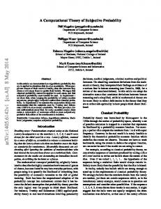
This thesis achieves a common framework for decision analysis and finite stage MDP’s by representing the MDP’s as decision networks. Since we have reinterpreted arcs into decision nodes as indications of both information availability and potential dependency, finite stage MDP’s can be naturally represented as decision networks. Figure 1.9 (1) depicts a three stage MDP in the graph-theoretical language of decision networks. We notice that there are no arcs from s1 and d1 to d2 even though s1 and d1 will be observed at the time the decision d2 is to be made. The

24


s

d1 1

s2

v1

d2

s

d3 3

s4

v3

v2 (1)

s

d1 1

v1

s2

d2

s

d3 3

v2

s4

v3 v

(2)

Figure 1.9: A three period finite stage MDP. reason is that the optimal decision rule for d2 is independent of s1 and d1 given s2 . However if we insist, as in influence diagrams, on interpreting arcs into decision nodes as indications of only information availability, then it is cumbersome to represent finite stage MDP’s. Figure 1.9 (2) depicts the influence diagram that represents the three stage MDP (Tatman and Shachter 1990). One can see that there is a number of extra no-forgetting arcs, namely arcs from s1 and d1 to d2 and d3 , and from s2 and d2 to d3 . The presence of those arcs not only complicates the network, but also fails to reflect one important conclusion of MDP, namely that the current decision is independent of previous states and decisions given the current state. Tatman and Shachter’s algorithm is able to detect that d2 does not depend on s1 and d1 , and that d3 does not depend on s1 , d1 , s2 , and d2 . So, the extra no-forgetting arcs makes no difference to the decision problem after all. They were introduced only because there was no concept of a decision network that does not satisfy the no-forgetting constraint. In a finite stage MDP, there is a reward in each period. This can be naturally


25

represented by assigning one value node for each period, as shown in Figure 1.9 (1). Note that s3 separates the last period from all the previous periods. If we insist, as in influence diagrams, on the single value node constraint, then we need to connect v1 , v2 , and v3 into a “super node” (Tatman and Shachter 1990), as shown in Figure 1.9 (2). One notices that no longer s3 separates the last period from all the previous periods. This is another reason for lifting the single value node constraint. 1.7

Computational merits

The lifting of the no-forgetting, regularity, and single value node constraints allows us to discover stepwise-decomposable decision networks (SDDN). SDDN’s are more general than both influence diagrams and finite stage MDP’s. Moreover when evaluating SDDN’s we can prune removable arcs, while the same cannot be done when evaluating influence diagrams since pruning arcs leads to the violation of the no-forgetting constraint. To put it more abstractly, SDDN’s relax constraints imposed by influence diagrams and thus allow us to apply more techniques in solving a problem, and hence to solve the problem more efficiently. See Sections 6.5 and 9.6.1. 1.8

Why not lifted earlier

Howard and Matheson (1984) have hinted that in the case of multiple decision makers, the regularity and no-forgetting constraints may be violated. Smith (1987) has also mentioned that it is possible that a decision maker may choose or be compelled to “forget”. Yet, no one before has studied decision networks that are not regular and/or are “forgetting”. Why?


26

Howard and Matheson (1984) deal only with regular and no-forgetting decision networks (influence diagrams), because for evaluation, decision networks are first transformed into decision trees, and the transformation is possible only for regular no-forgetting decision networks. Even though new algorithms for evaluating influence diagrams have been developed after Howard and Matheson (1984) (see, for example, Shachter 1986), the correctness of all those algorithms relies on the regularity and no-forgetting constraints. This is probably why those constraints have always been imposed on influence diagrams. In this thesis, we shall show that one can evaluate a decision network, even if it is not regular and no-forgetting. This opens up the possibility of working with general decision networks. 1.9

Subclasses of decision networks

The lifting of the no-forgetting, the regularity, and the single value node constraints from influence diagrams leaves us only with the acyclicity and no-children-to-value-node constraints. In Chapter 2, we shall argue that those two constraints are fundamental and can not be lifted. The acyclicity and no-children-to-value-node constraints define the concept of decision network. This section previews subclasses of decision networks we will encounter in this thesis. Influence diagrams and finite stage MDP’s are two existing subclasses of decision networks, which have been studied for many years. It is known that both of those subclasses of decision networks are stepwise-solvable, i.e they can be evaluated by considering one decision node at a time. The most important subclass of decision networks introduced in this thesis is stepwisedecomposable decision networks (SDDN). They include both influence diagrams and

27


abnormal decision networks

normal decision networks

regular SDDN’s

SDDN’s decision networks

finite stage MDP’s

influence diagrams

smooth decision networks non-smooth decision networks

Figure 1.10: Subclasses of decision networks. finite stage MDP’s as special cases. See Figure 1.10. SDDN’s are also stepwise-solvable. As a matter of fact, regular SDDN’s4 are the subclass of decision networks that can be evaluated by conventional dynamic programming (Denardo 1982, Chapter 9), and SDDN’s in general constitute the subclass of decision networks that can be evaluated by non-serial dynamic programming (Bertel`e and Brioshi 1972, Chapter 9). The decision networks that are not stepwise-decomposable can be of various degrees of decomposability. To evaluate them, one needs to simultaneously consider two or more decision nodes. The number of decisions one need to consider simultaneously is determined by the degree by which the network is decomposable. The divide and conquer strategy spelled out in Chapter 4 can be utilized to explore the decomposability of a given decision network. Smooth decision networks are introduced for technical convenience. They are conceptually simple and thus easy to manage. They are used extensively in this thesis to introduce new concepts and to prove theorems. Non-smooth decision networks can be 4

To be more precise, the term decision network should be replace by the term decision network skeleton in this section.


28

be transformed into equivalent smooth decision networks when necessary. Finally normal decision networks are introduced so that the equivalence between stepwise-decomposability and stepwise-solvability can be established. We conjecture that abnormal decision networks can be transformed into equivalent normal decision networks. 1.10

Who would be interested and why

Generally speaking, if you anticipate a solution to your problem by Bayesian decision theory, you should find this thesis interesting. Because it provides, in a sense, the most general framework — decision networks — for applying Bayesian decision theory. Problems representable as MDP’s can be solved in (stepwise-decomposable) decision networks in the same way as before. Problems representable in influence diagrams can be solved in (stepwise-decomposable) decision networks at least as efficiently as, and usually more efficiently, than in influence diagrams. The reason for this efficiency improvement is that working with SDDN’s relaxes the constraints imposed by influence diagrams, and allows one to apply more operations, such as pruning removable arcs, than previously allowed. If you are a decision analyst, you might appreciate the ability of decision networks to represent independencies for decision nodes, to accommodate multiple cooperative decision makers, and to handle multiple value nodes. You might find it a relief that you do not have to completely order the decision nodes beforehand. Furthermore, you might appreciate the efficiency and other advantages of our algorithms. If your problem falls into the category of MDP’s, you might find the concept of decision networks helpful in assessing the transition probabilities and rewards. In the ski retailer problem (Section 1.6), many factors may affect the transition probabilities and rewards, for example deterioration of stock, delivery lag, payment upon delivery by the retailer and by customers, refusal to enter backlog by customers (Denardo 1982).


29

Within MDP, one needs to figure out the dynamic programming functional equation for each combination of the factors, which may be complicated. In decision networks, consideration of one more factor simply corresponds to the addition of one more node. This allows one to consider more factors than before. The representation advantage of decision networks may benefit control theory in general. AI researchers who are concerned with planning, and diagnosis and treatment/repair should also find this thesis interesting. Planning is a process of constructing courses of action in response to some objective. Since the planner might not have complete knowledge about the environment and about the effects of actions, planning are usually performed under uncertainty. Being a theory for rational choice of actions under uncertainty, Bayesian decision theory naturally comes into play. Preliminary research (Dean and Wellman 1992) has indicated that successful application of Bayesian decision theory in planning under uncertainty calls for a framework that combines characteristics of influence diagrams and and those of MDP’s. Research on diagnosis and treatment (Provan and Clarke 1993) has pointed to the same direction. The concept of decision network introduced in this thesis may prove to be a good combination of influence diagrams and MDP’s. Also, the ability of decision networks to represent conditional independencies for decision nodes may be computationally essential for those areas.

Chapter 2

Decision networks: the concept

This chapter introduces the concept of decision networks and addresses some of the foundational issues. Formal definitions will be provided in Chapter 3. The concept of decision networks is intuitively illustrated through an example in section 2.1. Section 2.2 exposes the way by which other authors develop the concept of Bayesian networks from joint probabilities by means of the chain rule of probabilities, and by using the concept of conditional independencies. Section 2.3 derives the concept of decision network, through the concept of Bayesian networks, from the Bayesian decision theory setup by considering multiple decision problems. Section 2.4 discusses the fundamental constraints that decision networks need to satisfy and argues that decision networks are the most general representation framework for solving multiple-decision problems in Bayesian decision theory. 2.1

Decision networks intuitively

In this section, we illustrate the concept of decision networks through an example. Decision networks can be understood at two levels: relation and number. At the level of relation, decision networks are directed graphs consisting of three types of nodes: decision nodes, random nodes and value nodes; and they are used to graphically represent the structures of decision problems. This directed graph is called a decision network skeleton. Consider the further extended oil wildcatter problem:

30

Chapter 2. Decision networks: the concept

31

Figure 2.11: A decision network skeleton for the extended oil wildcatter problem. An oil wildcatter is deciding whether or not to drill in a new area. To aid his decision, he can order a seismic structure test. His decision about drill will depend on the test results if a test is ordered. If the oil wildcatter does decide to drill, crude oil and natural gas will be produced. Then, the oil wildcatter will decide his gas sale policy and oil sale policy on the basis of the quality and quantity of crude oil and natural gas produced, and on the basis of market information. The structures of this decision problem can be represented by the decision network skeleton shown in Figure 2.111 , where decision nodes are drawn as rectangles, random nodes as ovals, and value nodes as diamonds. Briefly, here are the semantics of a decision network. Arcs into random nodes indicate probabilistic dependencies. A random node depends on all its parents, and is independent 1

The figure is the same as Figure 1.8. The duplication is to save the reader from flipping back and forth.


32

of all its non-descendants given the values of its parents. In the extended oil wildcatter problem, test-result, for instance, probabilistically depends on seismic-structure and the decision to test, but is independent of gas-underground and oil-underground given seismic-structure and test. Arcs into decision nodes indicate both information availabilities and functional dependencies. In our example, the arc from oil-produced to oil-sale-policy means that the oil wildcatter will have learned the quantity and quality of crude oil-produced when he decides his oil-sale-policy, and he thinks that the quantity and quality of oilproduced should affect his oil-sale-policy. There is no arc from oil-underground to oil-sale-policy because information about oil-underground is not directly available. There is no arc from test-result to oil-sale-policy, because the oil wildcatter figures that the information about the test-result should not affect his oil-sale-policy since that he will already have learned the quality and quantity of crude oil-produced at the time the policy is to be made. Arcs into value nodes indicate functional dependencies. A value node is characterized by a function of its parents; the function take real number values, which represent the decision maker’s utilities. In the extended oil wildcatter problem, oil-sales is a function of oil-produced, oil-market and oil-sale-policy. It depends on no other nodes. For each possible values of oil-produced, of oil-market, and of oil-sale-policy, the value of this function stands for the corresponding expected oil-sales. The total utility is the sum of all the value nodes; namely the sum of test-cost, drill-cost, oil-sale and gas-sale. At the level of number, a decision network specifies a frame, i.e a set of possible values, for each variable. For example, the frame of drill my be {YES, NO}, and the frame of oil-sales may be the set of real numbers. There is also a conditional probability for each random node given its parents and prior


33

probability of each random node that does not have any parents. In our example, we need to specify, for instance, P (oil-underground), P (oil-produced|oil-underground), and etc . . . . Further, we need to specify a utility function for each value node. In our example, the utility function for oil-sales is a real function of oil-produced, oil-market, and oil-sale-policy. In summary, a decision network consist of (1) a skeleton which is an directed graph with three type of nodes, (2) a frame for each node, (3) a conditional probability for each random node, and (4) a utility or value function for each value node. In a decision network, the decision about a decision node is made knowing the values of the parents of the node. Optimal decisions are decisions that maximize the expected total utility. The goals of decision analysis are to find the optimal decisions and to determine the optimal expected total utility. 2.1.1

A note

Note that the term “decision network” has been previously used in Hastings and Mello (1977). The meaning of the term in this thesis is different. In this thesis, the nodes in a decision network are variables, while nodes in a Hastings and Mello decision network are states, or values of variables. In a sense, one can say that we are working at a higher level of abstraction than Hastings and Mello. The relationship between our decision networks and Hastings and Mello’s decision networks is the same as the relationship between influence diagrams and decision trees. As observed by Smith et al (1993), influence diagrams gain much of their advantages over decision trees from the fact that they graphically capture conditional independencies at the level of relation (among variables). The same can be said for our decision networks and Hastings and Mello’s decision networks. As the reader will see, the efficiency of our

34


algorithms heavily depends on the fact that nodes in our decision networks are variables, instead of values of variables. 2.2

Bayesian networks

One way to understand decision networks is to think of them as developed from the standard Bayesian decision theory setup. We shall explain this in the next section. As a preparation, this section develops the concept of Bayesian networks from joint probabilities by means of the chain rule of probabilities and the concept of conditional independency (Howard and Matheson 1984, Pearl 1988). Let X be a set of random variables. Let P (X) be the joint probability of the variables in X. It is usually difficult, if possible at all, to assess the joint probability directly. One way to assess the joint probability indirectly is first to choose an ordering over the variable set X, say x1 , x2 , . . . , xn , then to expand the joint probability by the chain rule as follows: P (x1 , x2 , . . . , xn ) = P (x1 )P (x2 |x1 ) . . . P (xn |x1 , . . . , xn−1 ).

(2.3)

We shall refer to the ordering as an expansion ordering . Because of equation (2.3), to assess the joint probability P (X), it suffices to assess P (xi |x1 , . . . , xi−1 ) for each i∈{1, . . . , n}. Often a decision maker is able to determine a proper subset πxi of {x1 , . . . , xi−1 } that are “directly related” to xi such that other variables in {x1 , . . . , xi−1 } are only “indirectly related” to xi via πxi . Translating into the language of the probability theory, this means that xi is independent of other variables in {x1 , . . . , xi−1 } given πxi . Formally that is P (xi |x1 , . . . , xi−1 ) = P (xi |πxi ). This equation further reduces the assessment task.

(2.4)

35


tampering

alarm

tampering

fire

smoke

leaving

(1)

Figure 2.12: Two Bayesian networks P (alarm, f ire, tampering, smoke, leaving).

fire

alarm

smoke

leaving

(2)

for

the

joint

probability

Given an expansion ordering x1 , . . . , xn and the πx′ i s, we construct a directed graph by the following rule: For any xi and xj , draw an arc from xi to xj if and only if xi ∈πxj . The acyclic directed graph such constructed, together with the conditional probabilities P (xi |πxi ), is called a Bayesian network for the joint probability P (X). As an example, consider the following decision scenario which is borrowed from (Poole and Neufeld 1991). The scenario involves five variables: alarm, fire, tampering, smoke, and leaving, denoting respectively the following propositions: the alarm is on, there is a fire, somebody is tampering; there is smoke and people are leaving. An expansion ordering for the joint probability P (alarm, fire, tampering, smoke, leaving) could be (fire, tampering, alarm, leaving, smoke). Suppose it is reasonable to set πtampering = ∅, πalarm = {fire, tampering}, πleaving = {alarm}, and πsmoke = {fire}. Then we get the Bayesian network shown in Figure 2.12 (1). Another expansion ordering could be (leaving, alarm, smoke, fire, tampering). Suppose it is reasonable to set πalarm = {leaving}, πsmoke = {alarm}, πfire = {alarm, smoke}, and πtampering = {fire, alarm}. Then we get the Bayesian network shown in Figure 2.12 (2). This network has more arcs than the one in (1).


36

How should one choose an expansion ordering? The answer provided by Howard and Matheson (1984) is that the ordering should be chosen such that the decision maker would feel natural and comfortable in assessing the πxi ’s and the P (xi |πxi )’s. For example, it probably is easier to assess P (alarm|fire, tampering) than to assess P (tampering|fire, alarm). Smith (1989) says that one should choose the ordering to minimize the number of arcs in the resulting directed graph. In our example, the network in Figure 2.12 (1) is preferred to the network in (2). Pearl (1988, pp. 50-51) claims that when there are cause-effect relationships among the variables, the structure of a Bayesian network can be directly determined from the cause-effect relationships. For example, tampering and fire cause alarm, fire causes smoke, alarm causes leaving. 2.3

Decision networks

In this section, decision networks are developed as a way to represent of the knowledge (beliefs) and utilities that are needed in order to solve multiple-decision problems in Bayesian decision theory. Let us begin with a standard setup of Bayesian decision theory. 2.3.1

A general setup of Bayesian decision theory

Here is a setup of Bayesian decision theory (G¨ardenfors et al 1988b, Fishburn 1988) that is more general than the one given in Section 1.2: 1. There is a set X of (random and decision) variables, which are relevant to a decision problem; 2. there is a set ∆ of policies and for each possible policy δ∈∆, there is a corresponding probability Pδ (X);

37


3. and there is a utility function µ(X), which specifies the decision maker’s preferences about the possible states of affairs. The problem is to decide on a policy δ 0 that maximizes the expected utility, that is X

Pδ0 (X)µ(X) = maxδ {

X

where

P

X

X

Pδ (X)µ(X)},

(2.5)

X

means summation over all the possible values of X.

The setup given in Section 1.2 can be fitted into the setup given here by letting X = {o, s, d}, and for each policy δ : O→Ωd setting Pδ (o, s, d) =

    

P (s)P (o|s)

if d = δ(o)

0

otherwise

(2.6)

In equation (2.5), summation is used instead of integration because we deal only with discrete variables in this thesis. However, most of our results can be easily extended to the case of continuous variables. 2.3.2

Multiple-decision problems

In applications, the decision maker usually needs to set the values for a number of variables d1 , . . . , dk . Let OBS(di) denote the set of all the variables whose values will be observed by the decision maker at the time of decision di is to be made. Sometimes, as in MDP’s, the decision maker is able to qualitatively tell that some of those observed variables are irrelevant to di . On other occasions, the decision maker may be forced, for instance by computational complexity, to approximate the world by by making such irrelevance assumptions. Let πd0i be a subset of OBS(di), such that the variables in OBS(di) − πd0i are, according to the decision maker, irrelevant to the decision di given πd0i .


38

Before one can solve a problem, one needs first to clearly state the problem. The concept of multiple-decision problems is introduced as a way to pose a decision problem. A multiple-decision problem is a set D = {< di, πd0i > |1 ≤ i ≤ k}, where the di ’s are decision variables and for each i, πd0i is the set of variables depending upon whose values the decision maker is to choose a value for di . The further extended oil wildcatter problem (Figure 2.11) is a multiple-decision problem. The decision maker needs to decide on a value for each of the following variables: test, drill, gas-sale-policy, and oil-sale-policy. The π 0 ’s are as follows: 0 0 0 πtest = ∅, πdrill = {test-result}, πgas −sale−policy = {gas-produced, gas-market}, 0 and πoil −sale−policy = {oil-produced, oil-market}.

Given a multiple-decision problem D, define a partial ordering among its variables as follows: for any two variables x and y, we say that x precedes y if x∈πyo , or if there is another variable z such that x∈πzo and z precedes y. The fundamental constraint that a multi-decision problem must obey is the so-called acyclicity constraint , which require that there do not exist two variables x and y such that both x precedes y and y precedes x. The reason for this constraint is that the precedence relationship defined above implies time precedence. More explicitly, if x precedes y, then the value of x is observed or determined before the value of y. 2.3.3

Technical preparations

Given a multiple decision problem D, let X be the set of all the variables in D and other variables that are relevant to the problem. For the further extended oil wildcatter problem, X also contains oil-underground, gas-underground, and seismic-structure in addition to the variables appeared in the problem statement, namely test, drill, gassale-policy, oil-sale-policy, test-result, gas-produced, gas-market, oil-produced, and oil-market.


39

For any variable x∈X, let Ωx be the frame of x, i.e. the set of all possible values of x. For any subset B ⊆ X, let ΩB =

Q

x∈B

Ωx .

To determine a value for di based on the values of the variables in πd0i is to choose a function δi : Ωπd0 → Ωdi . Such a function is called a decision function (table) for di . Let i

∆i denote the set of all the decision functions for di . The policy space is the Cartesian product ∆ = 2.3.4

Qk

i=1

∆i . An element of ∆ is called a policy .

Deriving the concept of decision networks

One needs to have the necessary knowledge to solve a problem. This subsection develops decision networks as a framework for specifying the knowledge (beliefs) and utilities that are required in order to solve a multiple-decision problem. If the decision maker wants to solve a multiple-decision problem D in the setup given in Subsection 2.3.1, then s/he needs, according to the second item of the setup, to come up with a probability Pδ (X) for each policy δ. When obtained, Pδ would contain more information than is conveyed by D and δ. The portion of information conveyed by Pδ that is not conveyed by D and δ should originate from the decision maker’s knowledge and beliefs about the uncertainties involved in the decision situation. Equipped with Bayesian networks, we are able to explicitly spell out this portion of information, as demonstrated in the following. Assume Pδ (X) were somehow obtained. An expansion ordering for Pδ (X) conforms to D if for each di , variables in πd0i precede di in the ordering. One can easily verify that such an ordering is possible since D must be acyclic. Given an expansion ordering ρ: x1 , . . . , xn that conforms to D, we could, as in the previous section, expand Pδ (X), determine the πxi ’s, and construct a Bayesian network. Denoted by Nδ , this Bayesian network would contain the following information:


40

1. For each decision node di , the conditional probability Pδ (di |πdi ) and the fact that (Fact1:) di is independent of all the variables that come before di in ρ given the variables in πdi ; and 2. for each random node c, the conditional probability Pδ (c|πc ) and the fact that (Fact2:) c is independent of all the variables that come before c in ρ given the variables in πc . Since πdi and πd0i have the same semantics, we have πdi =πd0i . Hence Fact1 would have come from the problem statement D; and the conditional probability Pδ (di |πdi ) would have come from the policy δ. One the other hand, Fact2 and the conditional probability Pδ (c|πc ) do not follow from either D or δ, and hence must have come from the decision maker. They represent the decision maker’s knowledge and beliefs about the uncertainties involved in the decision situation and need to be elicited before the decision problem D can be solved in Bayesian decision theory. We now turn to utility. According to item 3 in the setup of Subsection 2.3.1, the decision maker needs also to express his preferences about the possible state of affairs by a utility function µ(X). µ(X) can sometimes be decomposed into the sum of a number of components, each of which depends only on a number of variables. Suppose µ(X) decomposes into m components µ1 (Z1 ) + . . . + µm (Zm ), where Zi is the set of variable of which µi depends upon. Introduce a value variable vi for each µi , and attach vi to the Bayesian network Nδ by drawing arcs from each of the variables of Zi to vi . In the following, we shall write Zi as πvi , and µi (Zi ) as µvi (πvi ). To summarize the discussions above and in Subsection 2.3.2, the decision maker needs to do the following in order to solve a multiple-decision problem in Bayesian decision theory:


41

1. specify the decision variables whose values are to be to determined, and the random variables and value variables that are related to those decision variables; 2. for each decision variable di , specify the set πdi of observed variables whose values are relevant to di , 3. determine an ordering ρ among all the variables such that ρ conforms to the problem statement {< di , πd0i > |i}. Let ρ[< x] denote the set of nodes that come before x in the ordering ρ. 4. for each random variable c, specify a subset πc of ρ[< c] such that c is P (c|ρ[< c]) = P (c|πc ), and specify the conditional probability P (c|πc ); 5. for each value variable v, specify the subset πv of variables in ρ[< v] that v depends upon and specify the utility function µvi (πvi ). We call the collection of all the information specified in items 1, 2, 4, and 5 a decision network . Thus, a decision network represents the decision maker’s knowledge (beliefs) and preferences (utilities) that are needed in order to solve a multiple-decision problem in Bayesian decision theory. The ordering ρ is not included as part of the decision network because it can be arbitrary as long as it conforms to {< di , πd0i > |i}. Smith (1989) presents a way of developing the concept of influence diagrams (decision networks) in terms of the so-called third part semantics. In this section, the concept of decision networks has been developed directly from a standard setup of Bayesian decision theory without using the third part semantics. 2.3.5

An example

As an example, consider a decision scenario where a decision maker needs to decide whether to bring-umbrella in light of weather forecast. An additional variable, rain,

42


rain

forecast

bring umbrella

satisfaction

(1)

rain

forecast

bring umbrella

satisfaction

(2)

Figure 2.13: Two decision networks for the rain-and-umbrella problem. which takes the value “yes” if it does turn out to rain and “no” otherwise, is believed to be relevant to the decision and hence is included in our analysis. For each decision function δ : Ωforecast → Ωbring−umbrella , the decision maker needs to come up with a joint probability Pδ (rain, forecast, bring − umbrella). The expansion ordering rain, forecast, bring-umbrella conforms to the decision problem. If the decision maker’s utility — satisfaction — is a function of rain and bring-umbrella, then the decision network is as shown in Figure 2.13 (1). To complete the specification of this network, one needs to assess the prior probability of rain and the conditional probability for forecast given rain. One also needs to assess the utility function. The expansion ordering forecast, rain, bring-umbrella also conforms to the decision problem. It gives rise to the decision network shown on Figure 2.13 (2). The reader will see later that one can go between those two networks by reversing the arc between forecast and rain using Bayes’ theorem (see Howard and Matheson 1984 and Section 5.5). 2.4

Fundamental constraints

In the introduction we have seen that among the five constraints that define influence diagrams, the regularity, the no-forgetting, and the single value node constraints should be lifted. This short section considers the remaining two constraints, namely the acyclicity


43

and the no-children-to-value-node constraints. In the derivation of decision networks in the previous section, we first had a Bayesian network Nδ consisting of decision and random nodes. Then each value node v was attached to Nδ by drawing arc from those nodes in Nδ that v depends upon. Thus, the value nodes do not have children. In other words, decision networks always satisfy the no-children-to-value-node constraint. There is one issue that needs to be addressed. In the last section, we have assumed the set of value nodes does not intersect with the set of random and decision nodes. This may not be the case sometimes; there may be nodes that are value nodes and decision or random nodes at the same time. For example, the amount of money x one spends the next month is a value variable. In the meantime, x is also a decision variable, and it affects how much one will be willing to spend the month after. In such a case, we will have two copies of x: one copy xd functions as a decision node, while the other xv functions as a value node. Since xd is a decision node, one can set its value at his will and this value affects later decisions. On the other hand, the value node xv depends on xd and it does not affect any other nodes. By appropriately introducing copies of variables, we can always ensure that the set of value nodes does not intersect with the set of random and decision nodes. We now turn to consider the acyclicity constraint. Decision networks must always be acyclic because multiple-decision problems are acyclic (subsection 2.3.2) and Bayesian networks acyclic. In the derivation of the last section, we began with a joint probability Pδ (X) which one must have in order to solve the multiple-decision problem D in Bayesian decision theory. Because D is acyclic, we were able to have an expansion ordering ρ for Pδ (X) that conforms to D. The ordering ρ led to a Bayesian network Nδ . For any arc x→y in the Bayesian network, x comes earlier than y in the ordering ρ. Therefore Nδ must be acyclic. A decision network was obtained from Nδ by adding value nodes. Since


44

the value nodes do not have any children, the decision network must also be acyclic. The acyclicity and the no-children-to-value-node constraints are the only two constraints we impose on decision networks. We have just argued that those two constraints are fundamental and are indispensable to decision networks. In this sense, we say that decision networks are the most general representation framework for solving multipledecision problems in Bayesian decision theory.

Chapter 3

Decision networks: formal definitions

The previous chapter has introduced the concept of decision networks. This chapter gives the exact definitions. We first formally define Bayesian networks (Section 3.1) and give two properties of Bayesian networks that will be useful later in a number of places (Section 3.2). Then we present the formal definitions of decision networks and of their evaluation (Section 3.3). A naive algorithm for evaluating decision networks is provided in Section 3.4. This algorithm is very inefficient because it simultaneously considers all the decision nodes. A decision network is stepwise-solvable if it can be evaluated by considering one decision node at a time (Section 3.5). Obviously, stepwise-solvability is a desirable computational property. In the next three chapters, we shall discuss when a decision network is stepwise-solvable and how to evaluate a stepwise-solvable decision network. For that purpose, we need the auxiliary concept of semi-decision networks (Section 3.6). Starting from this chapter, we shall introduce various mathematical symbols. To help the reader to keep track of them, we have listed all the major symbols at the beginning of the thesis. 3.1

Formal definition of Bayesian networks

Before getting started, let us note that in this thesis, standard graph theory terms such as acyclic directed graphs, parents (direct predecessors), children (direct successors), predecessors, descendants (successors), leaves (nodes with no children), and roots (nodes 45

46

Chapter 3. Decision networks: formal definitions

a

a b

f

c

d

c

e

d e

g net1

b

b

net2

c

d e net3

Figure 3.14: Bayesian network and irrelevant variables. with no parents) will be used without giving the definitions. The reader is directed to Lauritzen et al (1990) for exact definitions. We shall use πx to denote the set of parents of a node x in a directed graph. A Bayesian network1 (Pearl 1988) N is a triplet N = (X, A, P), where 1. X is a set of random nodes (variables); each x∈X has a frame Ωx — the set of possible values of x; 2. A is a set of arcs over X such that (X, A) is an acyclic directed graph; and 3. P is a set {P (x|πx )|x ∈ X}2 of conditional probabilities of the variables given their respective parents3 . Figure 3.14 show a simple Bayesian network net1 with seven variables a, b, c, d, e, f , and g. The network contains the following prior and conditional probabilities: P (a), P (f |a), P (b|a), P (c|b), P (d|b), P (e|c, d), and P (g|f, e). 1

Bayesian networks are also known as belief networks, Bayesian belief networks, and probabilistic influence diagrams. 2 P A conditional probability P (x|πx ) is a mapping P (x|πx ) : Ω{x}∪πx → [0, 1] such that ωx ∈Ωx P (x=ωx |πx =β) = 1 for each value β of πx . 3 When x is a root, πx is empty. When it is the case, P (x|πx ) stands for the prior probability of x.

47


The prior joint probability PN (X)4 of a Bayesian network N = (X, A, P) is defined by PN (X) =

Y

P (x|πx ).

(3.7)

x∈X

In words, PN (X) is the pointwise multiplication of all the conditional probabilities in N . For any subset B ⊆ X, the marginal probability P (B) is defined by P (B) =

X

P (X),

(3.8)

X−B

where

P

X−B

means summation over all the possible values of the variables in the set

X−B. A note about notation usage: In equation (3.7) the range of the multiplication is specified by the sign “∈”; x∈X means x ranges over X. In equation (3.8) there is no “∈” sign. As a convention, we use

P

X−B

P (X) as an abbreviation of

P

ωX−B ∈ΩX−B

P (ωB , ωX−B ),

where ωX−B stands for a general member of ΩX−B , ωB stands for a general member of ΩB , and (ωB , ωX−B ) is thus a general member of ΩX . We shall always follow this convention about notation usage throughout this thesis. For any two subsets B1 , B2 ⊆ Y of variables, the conditional probability P (B1 |B2 ) is a function that satisfies P (B1 =β1 , B2 =β2 ) = P (B2 =β2 )P (B1 =β1 |B2 =β2 ) ∀β1 ∈ΩB1 , ∀β2 ∈ΩB2 .

(3.9)

For technical convenience, we also introduce the auxiliary concept of semi-Bayesian networks. A semi-Bayesian network is a Bayesian network except that the prior probabilities of some of the root nodes are missing. More precisely, a semi-Bayesian network is a quadruplet N = (X, A, P|S), where (X, A) is a acyclic directed graph, P = {P (x|πx )|x∈X−S} is set of conditional probabilities, and S is the set of root nodes whose prior probabilities are missing. 4

A function from ΩX to [0, 1].

48


It follows from the definition that Bayesian networks are semi-Bayesian networks. As in Bayesian networks, we can define PN (X) as follows, PN (X) =

Y

P (x|πx ).

(3.10)

x∈(X−S)

Unlike in Bayesian networks, here PN (X) usually is not a probability; it may not sum to one. Thus, it is called the prior joint potential instead of the prior joint probability. Marginal and conditional potentials can be defined from the joint potential in the same way as marginal probabilities are defined from joint probabilities. Note that since there are no arcs from X−S to S, the prior joint potential PN (X) is nothing but the conditional probability of the variables in X−S given variables in S. For example, net3 in Figure 3.14 is a not Bayesian network if we have only P (c|b), P (d|b), and P (e|c, d) but not P (b). In this case, net3 is a semi-Bayesian network. The multiplication of all the conditional probabilities yields the conditional probability P (c, d, e|b). 3.2

Variables irrelevant to a query

Given a (semi-)Bayesian network N , one can pose a query ?PN (B1 |B2 ). It is often possible to graphically identify certain variables being irrelevant to the query ?PN (B1 |B2 ). This issue is addressed in Geiger et al (1990), Lauritzen et al (1990), and Baker and Boult (1990). The materials in the reminder of this section are extracted from those papers. To remove a node x from a semi-Bayesian network N = (X, A, P|S) is to: (1) remove x from X, (2) remove from A all the arcs that contain x, (3) remove from P all the items that involve x, and (4) those nodes that were not roots and become roots because of the removal are added to S. We notice that removing a node from a Bayesian network may create root nodes which do not have prior probabilities. This is why we need the concept of semi-Bayesian network.


49

A leaf node is barren w.r.t a query ?PN (B1 |B2 ), if it is not in B1 ∪B2 . In net1 (Figure 3.14), g is barren w.r.t ?Pnet1 (e|b). The following proposition says that if a leaf node is barren w.r.t a query, then it is irrelevant to the query, and hence can be harmlessly removed. Lemma 3.1 Suppose N is a semi-Bayesian network, and x is a leaf node. Let N ′ be the semi-Bayesian network obtained from N by removing x. If x is barren w.r.t to the query ?PN (B1 |B2 ), then PN (B1 |B2 ) = PN ′ (B1 |B2 ).

(3.11)

Consider computing Pnet1 (e|b). The node g is barren w.r.t the query and hence irrelevant. According to Lemma 3.1, g can be harmlessly removed. This creates a new barren node f . After the removal of g and f , net1 becomes net2. Thus the query ?Pnet1 (e|b) is reduced to the query ?Pnet2 (e|b = b0 ). Let An(B1 ∪B2 ) be the ancestral set of B1 ∪B2 , i.e the set of nodes in B1 ∪B2 and the ancestors of those nodes. By repeatedly applying Lemma 3.1, we get Proposition 3.1 All the nodes outside An(B1 ∪B2 ) are irrelevant to the query ?P (B1 |B2 ). Let G = (X, A) be a directed graph. An arc from x to y is written as an ordered pair (x, y). The moral graph m(G) of G is an undirected graph m(G) = (X, E) whose edge set E is given by E = {{x, y}|(x, y) or (y, x) ∈ A, or ∃z such that (x, z) and (y, z) ∈ A}. In words, {x, y} is an edge in the moral graph if either there is an arc between the two vertices or they share a common child. The term moral graph was chosen because two nodes with a common child are “married” into an edge (Lauritzen and Spiegehalter 1988).

50


In an undirected graph, two nodes x and y are separated by a set of nodes S if every path connecting them contains at least one node in S. In a directed graph G, x and y are m-separated by S if they are separated by S in the moral graph m(G)5 . Note that any node set separates itself from any other set. Proposition 3.2 Suppose N is a semi-Bayesian network. Let N ′ be the semi-Bayesian network obtained from N by removing all the nodes that are not in B2 and are m-separated from B1 by B2 . Then PN (B1 |B2 ) = PN ′ (B1 |B2 ).

(3.12)

In our example, since a is m-separated from e by b in net2, the query can be further reduced to Pnet3 (e|b). Note that a is not m-separated from e by b in net1. It can be proved (Lauritzen et al 1990 and Geiger et al 1990) that all the nodes irrelevant to a query ?PN (B1 |B2 ) can be recognized and removed by applying Proposition 3.1 and Proposition 3.2. 3.3

Formal definitions of decision networks

A decision network skeleton is an acyclic directed graph K = (Y, A), which consists of three types of nodes: random nodes, decision nodes, and values nodes; and where the value nodes have no children. A decision network skeleton describes a decision problem at the level of relation. It contains the set of parents πd for each decision node d, the set of parents πc for each random nodes, and the set of parents πv for each value nodes. See Subsection 2.3.4. A decision network N is a quadruplet N =(Y, A, P, F ) where 5

To relate m-separation to d-separation (Pearl 1988), Lauritzen et al (1990) have shown that S d-separates B1 and B2 if and only if S m-separates B1 and B2 in the ancestral set An(B1 ∪S∪B2 ).

51


1. (Y, A) is a decision network skeleton. Let us use C to denote the set of random nodes, D to denote the set of decision nodes, and V to denote the set of value nodes. 2. Each y∈Y has a frame Ωy — the set of possible values of y. 3. P is a set {P (c|πc )|c∈C} of conditional probabilities of the random nodes given their respective parents. 4. F is a set {µv : Ωπv →R1 |v∈V } of value (utility) functions for the value nodes, where R1 stands for the real line. A decision network is obtained from a decision network skeleton by providing numerical information, i.e by specifying a frame for each variable, providing a conditional probability of each random node, and a value function for each value node. We say that (Y, A, P, F ) is a decision network over the skeleton (Y, A) , and that (Y, A) is the skeleton of the decision network (Y, A, P, F ). A decision function (table) for a decision node di is a mapping δi : Ωπdi → Ωdi . The decision function space ∆i for di is the set of all the decision functions for di . Let D = {d1 , . . . , dk } be the set of all the decision nodes. The Cartesian product ∆ =

Qk

i=1

∆i

is called the policy space for N , and a member δ=(δ1 , . . . , dk ) ∈ ∆ is called a policy . Note that while a decision function δi is a function, a policy δ is a vector of decision functions. The relationship between a decision node di and its parents πdi as indicated by a decision function δi : Ωπdi → Ωdi is equivalent to the relationship as represented by the conditional probability Pδi (di |πdi ) given by Pδi (di =α|πdi =β) =

    

1 if δi (β)=α 0 otherwise,

(3.13)

52


for all α∈Ωdi and β∈Ωπdi . Since δ=(δ1 , . . . , δk ), we sometimes write Pδ (di |πdi ) for Pδi (di |πdi ). Because of equation (3.13), we will abuse the symbol δ by letting it also denote the set {Pδ (di |πdi )|di ∈D} of conditional probabilities of the decision nodes. In a decision network N =(Y, A, P, F ), let X=C∪D. Let AX be the set of all the arcs of A that lie completely in X. Then the triplet (X, AX , P∪δ) is a Bayesian network, where δ denotes a set of conditional probabilities of the decision nodes. We shall refer to this Bayesian network the Bayesian network induced from N by the policy δ, and write it as Nδ . The prior joint probability Pδ (X) of Nδ is given by Pδ (X) =

Y

P (x|πx )

x∈C

Y

Pδ (x|πx ).

(3.14)

x∈D

We shall refer to Pδ (X) as the joint probability over X induced by δ . Because the value nodes do not have children, for any value node v, πv contains no value nodes. Hence πv ⊆X. The expectation Eδ [v] of the value function µv (πv ) of v under Pδ is given by Eδ [v] =

X

Pδ (X)µv (πv )

X

Pδ (πv )µv (πv ).

X

=

(3.15)

πv

The expected value Eδ [N ] of N under the policy δ is defined by Eδ [N ] =

X

Eδ [v]

X

Pδ (X)

(3.16)

v∈V

=

X

Let us point it out again that

P

of πv and X respectively, while

πv

P

for a note about notation usage.

and v∈V

P

X

X

µv (πv ).

(3.17)

v∈V

mean summation over all the possible values

means summation over the set V . See Section 3.1

53


The optimal expected value E[N ] of N is defined by E[N ] = maxδ∈∆ Eδ [N ].

(3.18)

The optimal value of a decision network that does not have any value nodes is zero. An optimal policy δ o =(δ1o , . . . , δko ) is one that satisfies Eδo [N ] = E[N ].

(3.19)

We call δio an optimal decision function (table) of di . For a decision network that does not have any value nodes, all policies are optimal. In this thesis, we shall only consider variables with finite frames. Hence there are only finitely many possible policies. Consequently, there always exists at least one optimal policy. To evaluate a decision network is to 1. find an optimal policy, and 2. find the optimal expected value. 3.4

A naive algorithm

A straightforward approach to the evaluation of decision networks is to simply follow the definitions of optimal policy and of optimal expected value, and exhaustively search through the policy space ∆. This idea is made explicit by the following algorithm. Procedure NAIVE-EVALUATE: • Input: N — a decision network. • Output: An optimal policy and the optimal expected value of N .

54


Let ∆ be the policy space of N . 1. Pick one policy from ∆ and denoted it by δ o . Set ∆ = ∆−{δ o }. 2. Compute Eδo [N ]. 3. While ∆ 6= ∅, do • Pick one policy from ∆ and denoted if by δ. Set ∆ = ∆−{δ}. • Compute Eδ [N ]. • If Eδ [N ] > Eδo [N ], set δ o = δ. end-while 4. Output δ o and Eδo [N ]. Though simple, this naive algorithm is very inefficient. The main reason is that it simultaneously considers all the decision nodes. This results in an exhaustive search through the policy space ∆, which can be computationally prohibitive. Suppose there are k decision nodes, each has l parents, and suppose all the variables are binary. Then l

for each decision node d, the cardinality of Ωπd is 2l ; hence there are 2(2 ) possible decision l

functions for d. Consequently there are (2(2 ) )k policies in ∆. The procedure NAIVEl

EVALUATE computes the expected value of N for each of the (2(2 ) )k policies! There are decision networks whose evaluation necessitates simultaneous consideration of all the decision nodes. As an example, consider the decision network (skeleton) in Figure 3.15. Enemy movements may be observed by both agent1 and agent2. An agent decides whether or not to report enemy movements according to the instructions established beforehand by the intelligence office. If an agent reports, there is a chance that s/he may be exposed.

55


enemy movement observed by agent2

observed by agent1

agent1 reports

agent2 reports

agent2 exposed

agent1 exposed value

Figure 3.15: A decision network whose evaluation may require simultaneous consideration of all the decision nodes. For the sake of illustration, assume all the variables either take the value YES or NO, except for the variable value, which takes real numbers. To complete the specification, we need to give the following (conditional) probabilities: P (enemy-movement), P (observed-by-agent1|enemy-movement), P (observed-by-agent2|enemy-movement), P (agent1-exposed|agent1-reports), and P (agent2-exposed|agent2-reports). We need also to give value function µvalue (enemy-movement, agent1-exposed, agent2-exposed). There are four possible instructions (decision functions) for agent1: 1. If observed-by-agent1=YES, then agent1-reports=YES; If observed-by-agent1=NO, then agent1-reports=YES. 2. If observed-by-agent1=YES, then agent1-reports=YES; If observed-by-agent1=NO, then agent1-reports=NO. 3. If observed-by-agent1=YES, then agent1-reports=NO; If observed-by-agent1=NO, then agent1-reports=YES.

56


4. If observed-by-agent1=YES, then agent1-reports=NO; If observed-by-agent1=NO, then agent1-reports=NO. Similarly, there are four possible instructions for agent2. The policies (instructions for both agents) for the problem are given as follows: 1. If observed-by-agent1=YES, then agent1-reports=YES; If observed-by-agent1=NO, then agent1-reports=YES. and If observed-by-agent2=YES, then agent2-reports=YES; If observed-by-agent2=NO, then agent2-reports=YES. 2. If observed-by-agent1=YES, then agent1-reports=YES; If observed-by-agent1=NO, then agent1-reports=NO. and If observed-by-agent2=YES, then agent2-reports=YES; If observed-by-agent2=NO, then agent2-reports=YES. 3. and so on . . . 1

One can easily see that the policy space consist of (2(2 ) )2 = 4 ∗ 4 = 16 possible policies. In assessing his utilities, the intelligence office needs to keep both agents in mind. For example, it may be the case that information about an particular enemy movement is important enought to risk one agent but not both. The instructions for such a situation should allow one and only one agent to report. The instructions can require, for instance, agent1 to report when the information is deemed important enough to risk one agent, and require agent2 to report only when the information is deemed important enough to risk both agents. Such instructions can be arrived at only by considering the two agents


57

simultaneously. In Chapter 8, we shall formally prove that with appropriate probabilities and value functions, optimal policies for the decision network in Figure 3.15 can be found only by considering the two decisions at the same time. On the other hand, however, there are decision networks which allow more efficient algorithms than NAIVE-EVALUATE. The best case is when a decision network can be evaluated by considering one decision node at a time. This leads to the concept of stepwise-solvability. 3.5

Stepwise-solvability

Let N be a decision network. Let d1 , d2 , . . . , dk be all the decision nodes in N , and let δ=(δ1 , δ2 , . . . , δk ) be a policy of N , where δj is a decision function of dj . The expected value Eδ [N ] = E(δ1 ,δ2 ,...,δk ) [N ] is a function of δ1 , δ2 . . . , and δk . For any i∈{1, 2, . . . , k}, if we fix the value of δj for all j∈{1, 2, . . . , k} such that j6=i, then E(δ1 ,...,δi−1 ,δi ,δi+1 ,...,δk ) [N ] becomes a function of δi . Rank all the possible values of δi , i.e all the possible decision functions of di , according to the value E(δ1 ,...,δi−1 ,δi ,δi+1 ,...,δk ) [N ]. If the decision function (for di) that is ranked the highest remains the same regardless of the values of the δj ’s (j6=i), then we say that di is a stepwise-solvability candidate node , or simply an SS candidate node of N . A deterministic node is a random node whose conditional probability takes the value either 0 or 1. To replace a decision node dj by a deterministic node characterized by a function δj : Ωπdj → Ωd (Shachter 1988) is to replace dj by a deterministic node with the same frame, and to set P (dj |πdj ) to be the conditional probability that represents δj in the sense of equation (3.13). If di is an SS candidate node, then an optimal decision function δio can be found as follows. For all j∈{1, 2, . . . , k} such that j6=i, replace the decision node dj by a

58


deterministic random node characterized by an arbitrary decision function δj , resulting in a decision network with only one decision node di . Then find a policy δio of di that satisfies E(δ1 ,...,δi−1 ,δio ,δi+1 ,...,δk ) [N ] = maxδi ∈∆i E(δ1 ,...,δi−1 ,δi ,δi+1 ,...,δk ) [N ].

(3.20)

Proposition 3.3 If di is an SS candidate node of a decision network N , then an decision function δio that satisfies equation (3.20) is an optimal decision function of di . ∗ ∗ Proof: Let (δ1∗ , . . . , δi−1 , δi∗ , δi+1 , . . . , δk∗ ) be an optimal policy of N . Since di is an SS

candidate node and δio satisfies (3.20), we have ∗ ,δ o ,δ ∗ ,...,δ ∗ ) [N ] ≥ E(δ ∗ ,...,δ ∗ ,δ ∗ ,δ ∗ ,...,δ ∗ ) [N ]. E(δ1∗ ,...,δi−1 1 i−1 i i+1 i i+1 k k

∗ ∗ Therefore, (δ1∗ , . . . , δi−1 , δio, δi+1 , . . . , δk∗ ) must also be an optimal policy of N . Conse-

quently, δio must be an optimal decision function of di . The proposition is proved. 2 A decision network is stepwise-solvable if it contains no decision nodes, or if 1. there exists an SS candidate node di such that 2. if di is replaced by a deterministic node characterized by an optimal decision function of d, the resulting decision network (with one less decision node) is stepwisesolvable. A decision network skeleton is stepwise-solvable if all the decision networks over the skeleton are stepwise-solvable. If a decision network N is stepwise-solvable, then it can be evaluated as follows. Find an SS candidate node di and find an optimal decision function δio of di in the way as specified in equation (3.20). Replace di by a deterministic node characterized by δio , resulting in another stepwise-solvable decision network N ′ with one less decision node.

59


Then recursively apply the procedure to N ′ , an so on so forth. We see here that N is evaluated by considering one decision node at a time. Suppose N is a stepwise-solvable decision network with k decision nodes. Suppose each decision node has l parents, and suppose all the variables are binary. Then to l

evaluate N , we need to compute the expected values of N for (2(2 ) ) ∗ k policies, instead l

of (2(2 ) )k policies as in the case of NAIVE-EVALUATE. l

Note that the aforementioned evaluation method is not the best. The term 2(2 ) can easily be prohibitively large. We shall show that when a decision network is stepwisesolvable, it can be solved not only by considering one decision node at a time, by also by considering one, usually small, part of the network at a time. The complexity can be reduced to that of computing no more than 2k + m marginal probabilities of no more than l + 1 variables or computing no more than (2k + m)2l+1 numbers, where m stands for the number of value nodes. So, stepwise-solvability is a very desirable property for a decision network to possess. In the next three chapters, we shall investigate when a decision network is stepwisesolvable and what is the best way to evaluate a stepwise-solvable decision network. For this purpose, we need the technical concept of semi-decision network. 3.6

Semi-decision networks

The reader has seen that removing nodes from a Bayesian network may create root nodes which do not have prior probabilities. This is why we need the concept of semi-Bayesian network. We shall also be discussing removing nodes from decision networks, which necessitates the concept of semi-decision networks. A semi-decision network is a decision network except that the prior probabilities of some of the root random nodes are missing. We use N = (Y, A, P, F |S) to denotes a

60


semi-decision network, where S is the set of root random nodes whose prior probabilities are missing. As before, let X = C ∪ D be the set of random and decision nodes. Similarly to the case of decision networks, a policy δ induces a semi-Bayesian network (X, AX , P∪δ|S), which will be referred to as the semi-Bayesian network induced from N by the policy δ , and which will be written as Nδ . Let Pδ (X) be the prior joint potential of Nδ . For any value node v∈V , πv ⊆X. The expected value Eδ [N ] of N under the joint potential Pδ (X) is defined by X

Eδ [N ] =

Pδ (X)

X

X

µv (πv ).

(3.21)

v∈V

The optimal expected value E[N ] of N is defined by E[N ] = maxδ∈∆ Eδ [N ]. An optimal policy δ o is one that satisfies Eδo [N ] = E[N ]. Unlike in the case of decision networks, we also define the concept of conditional expected value for semi-decision networks. Th conditional expected value Eδ [N |S] of N given S is defined by Eδ [N |S] =

X

X−S

Pδ (X)

X

µv (πv ).

(3.22)

v∈V

Obviously Eδ [N |S] is a function of S. We chose the term “conditional expected value” because that the prior joint potential PN (X) is nothing but the conditional probability of the variables in X−S given S (see the note at the end of Section 3.1) . The optimal conditional expected value E[N |S] of N given S is defined by


61

E[N |S] = maxδ∈∆ Eδ [N |S]. An optimal conditional policy δ o is one that satisfies Eδo [N |S] = E[N |S], for all possible values of S. Proposition 3.4 A conditionally optimal policy of a semi-decision network, if exits, is always an optimal policy. Proof: From equations (3.21) and (3.22), we have Eδ [N ] =

X

Eδ [N |S].

S

Let δ o be a conditional optimal policy and let δ be an arbitrary policy of N . Then Eδo [N ] =

X

Eδo [N |S] ≥

S

X

Eδ [N |S] = Eδ [N ].

S

Therefore Eδo [N ] ≥ maxδ∈∆ Eδ [N ]. In words, δ o is an optimal policy of N . 2 For a semi-decision network, there always exists at least one optimal policy. But there may not necessarily exist any conditional optimal policies. Given a semi-decision network N , if every optimal policy of N is also a conditionally optimal policy, then we say that N is uniform . We shall investigate when a semi-decision network is uniform later.

Chapter 4

Divide and conquer in decision networks

This chapter and the next two chapters constitute the heart of this thesis; they introduce and study one subclass of decision networks, namely stepwise-decomposable decision networks (SDDN’s). SDDN’s are important because they are stepwise-solvable, and as we shall show in Chapter 8 stepwise-decomposability is the weakest graph-theoretical criterion that guarantees stepwise-solvability. This chapter investigates when and how a decision network can be decomposed into two subnetworks such that the optimal expected value and an optimal policy of the decision network can be computed by evaluating the two subnetworks. The next two chapters are concerned with how to evaluate decision networks that can be decomposed into n — the number of decision nodes — subnetworks such that the optimal expected values and optimal policies of the decision networks can be computed by evaluating the n subnetworks. The organization of this chapter is as follows. Section 4.1 discusses the relationship between independence in a decision network and separation in the underlying decision network skeleton. Section 4.2 defines a concept of decomposability for decision networks, and Section 4.3 shows that this concept of decomposability implies a divide and conquer evaluation strategy. Since manipulation of decision networks gives rise to semi-decision networks and decision networks are special semi-decision networks, exposition in this chapter will be carried out in terms of semi-decision networks. 62

63

Chapter 4. Divide and conquer in decision networks

YI

XI

πd

X II

YII

Figure 4.16: The relationships among the sets Y , YI , YII , XI , XII , and πd . The three sets YI , YII and πd constitute a partition of Y — the set of all the nodes; while XI , XII and πd constitute a partion of C∪D — the set of all the random and decision nodes. When the network is smooth at d, there are no arcs going from XII to πd . 4.1

Separation and independence

The main goal of this chapter is to prove Theorem 4.1, one of the most important theorems in this thesis. In preparation, this section exposes the relationship between graphtheoretic separation and probabilistic independence in the context of decision networks. Suppose K = (Y, A) is decision network skeleton and d is a decision node in K. Let YI (d, K), or simply YI be the set of all the nodes that are m-separated from d by πd , with the nodes in πd itself excluded. Let YII (d, K), or simply YII be the set of all the nodes that are not m-separated from d by πd . We observe that YI , πd , and YII forms a partition of Y . Let XI (d, K) = YI (d, K)∩(C∪D) and XII (d, K) = YII (d, K)∩(C∪D). The relationships among the sets are illustrated in Figure 4.16. In the following, we shall refer to YI as the upstream set of πd , YII as the downstream set of πd . We shall also refer to XI as the set of random and decision nodes in the upstream of πd , and XII as the set of random and decision nodes in the downstream of πd . Consider a semi-decision network N = (Y, A, P, F |S). Let δ be a policy of N . As pointed out by Lauritzen et al (1990), m-separation in the skeleton (Y, A) implies conditional independence for Pδ (X) — the joint potential over X induced by δ. Since πd

64


m-separates XI and XII , we have that Pδ (XII |XI , πd ) = Pδ (XII |πd ). Therefore Pδ (XI , πd , XII ) = Pδ (XI , πd )Pδ (XII |XI , πd ) = Pδ (XI , πd )Pδ (XII |πd ).

(4.23)

The rest of this section seeks an explicit representation of Pδ (XI , πd ) and Pδ (XII |πd ) in terms of conditional probabilities. A decision network is smooth at the decision node d, if there are no arcs going from the downstream set YII of πd to nodes in πd . In other words, arcs between πd and YII only go from πd to YII . As an example, consider the decision network skeleton for the further extended oil wildcatter problem (Figure 2.11). The downstream set of πoil−sale−policy consists of oil-sale-policy and oil-sales.

There are no arcs from oil-sales to nodes in

πoil−sale−policy . So, the skeleton is smooth at oil-sale-policy. One the other hand, the downstream set of πdrill contains all the nodes except test-cost and the nodes in πdrill . In particular, the downstream set contains the node seismic-structure. Because of the arc from seismic-structure to test-result (∈ πdrill ), the decision network skeleton is not smooth at drill. Let d1 , . . . , dj be all the decision nodes in XI ∪πd and dj+1, . . . , dk be all the decision nodes in XII . Note that d ∈ {dj+1, . . . , dk }. For a policy δ = (δ1 , . . . , δk ), let δI = (δ1 , . . . , δj ) and δII = (δj+1 , . . . , δk ). Suppose the semi-decision network N is smooth at d. It follows from Proposition 3.1 that Pδ (XI , πd ) =

Y

P (x|πx )

x∈C∩(XI ∪πd )

j Y

Pδi (di |πdi ).

(4.24)

Pδi (di |πdi )).

(4.25)

i=1

And it follows from Proposition 3.2 that Pδ (XII |πd ) =

Y

x∈C∩XII

P (x|πx )

k Y

i=j+1


65

Those two equations give us the following lemma. Lemma 4.1 If N is smooth at d, then Pδ (XI , πd ) only depends on δI , and Pδ (XII |πd ) only depends on δII . From now on, we shall write Pδ (XI , πd ) as PδI (XI , πd ), and Pδ (XII |πd ) as PδII (XII |πd ). 4.2

Decomposability of decision networks

Also in preparation for Theorem 4.1, this section introduces a concept of decomposability for decision networks and shows how to divide a decomposable decision network into two subnetworks. A decision network skeleton K=(Y, A) is decomposable at a decision node d if the number of decision node in YII (d, K) is less than the number of decision nodes in K. A semi-decision network is decomposable at a decision node d if the underlying skeleton is. When a decision network skeleton K is decomposable and smooth at d, we define the downstream component of K w.r.t d, denoted by KII (d, K) or simply KII , to be the decision network skeleton obtained by restricting K to πd ∪YII and then removing those arcs that connect two nodes in πd . Also, we define the upstream component of K w.r.t d, denoted by KI (d, K) or simply KI , to be the decision network skeleton obtained by restricting K to YI ∪πd and then adding a node u and drawing an arc from each node in πd to u. The node u is to be used to store the value of the downstream component, and is thus called the downstream-value node . Figure 4.17 shows the downstream and upstream components, w.r.t oil-sale-policy, of the decision network skeleton in Figure 2.11. Note that while YI and YII are sets of nodes, KI and KII are decision network skeletons. KI and KII contain the nodes in πd , while YI and YII do not.


66

Let N be a decision network over K, and suppose N (or K) is decomposable and smooth at d. The downstream component of N w.r.t d, denoted by NII (d, N ) or simply by NII , is a semi-decision network over KII . The value functions for all the value nodes of NII remain the same at in N . The conditional probabilities of the random nodes of NII that lie outside πd also remain the same as in N . The nodes in πd , random or decision, are viewed in NII as random nodes whose prior probabilities are missing. The upstream component of N w.r.t d, denoted by NI (d, N ) or simply by NI , is a semi-decision network over KI . The conditional probabilities of all the random nodes remain the same as in N . The values functions of the value nodes other than u also remain the same as in N . The value function µ(πd ) of the downstream-value node u is the optimal conditional expected value E[NII |πd ] of the downstream component NII . Since the decision node d is not in the upstream component NI , the number of decision nodes in NI is less than the number of decision nodes in N . Since the decision nodes in πd , if any, are treated as random nodes in NII and since the N decomposes at d, the number of decision nodes in NII is also less than the number of decision nodes in N . Furthermore the number of decision nodes in NI plus the number of decision nodes in NII equals the number of decision nodes in N . We shall later define the concepts of downstream and upstream components for the case when K and N are not smooth at d. 4.2.1

Properties of upstream and downstream components

This subsection gives several properties of upstream and downstream components of decomposable decision networks. Those properties will be useful in the proof of Theorem 4.1. Given a policy δII = (δj+1 , . . . , δk ), the downstream component NII is a semi-Bayesian network. Let PNII ,δII (πd , XII ) denote the prior joint potential of this semi-Bayesian

67



gas sales

gas produced

gas sale policy

test cost seismic structure

test

drill cost

drill test result

u oil underground

oil produced oil market

upstream component

oil produced

oil sale policy oil sales oil market

Downstream component

Figure 4.17: Downstream and upstream components: The downstream component is a semi-decision network, where the prior probabilities for oil-produced and oil-market are missing. In the upstream component, u is the downstream-value node, whose value function is the optimal conditional expected value of the downstream component. network. From the definition of the downstream component, one can see that if N is smooth at d, then PNII ,δII (πd , XII ) =

Y

P (x|πx )

x∈C∩XII

k Y

Pδi (di |πdi )),

i=j+1

which is the same as the right hand side of equation (4.25). Therefore we have Lemma 4.2 Suppose a semi-decision network N is decomposable and smooth at decision node d. Let PδII (XII |πd ) be as in Lemma 4.1. Then PNII ,δII (πd , XII ) = PδII (XII |πd ).

(4.26)

Similarly, given a policy δI = (δ1 , . . . , δj ), the upstream NI is a Bayesian network. Let PNI ,δI (XI , S) denote the joint probability of this Bayesian network. From the definition of the upstream component, one can see that if N is smooth at d, then

68


Y

PNI ,δI (XI , S) =

P (x|πx )

j Y

Pδi (di |πdi ),

i=1

x∈C∩(XI ∪πd )

which is equal to the right hand side of equation (4.24). Therefore we have Lemma 4.3 Suppose a semi-decision network N is decomposable and smooth at decision node d. Let PδI (XI , πd ) be as in Lemma 4.1. Then PNI ,δI (XI , πd ) = PδI (XI , πd ).

(4.27)

The following proposition is especially important to the proof of Theorem 4.1. Proposition 4.1 Suppose a semi-decision network N is decomposable and smooth at decision node d. Let PδII (XII |πd ) and PδI (XI , πd ) be as in Lemma 4.1. Let VI and VII be the set of value nodes in NI an NII respectively. Then the conditional expected value of NII under policy δII satisfies EδII [NII |πd ] =

X

PδII (XII |πd )

XII

X

µv (πv ),

(4.28)

v∈VII

and the expected value of NI under policy δI satisfies EδI [NI ] =

X

PδI (XI , πd ){

XI ,πd

X

µv (πv ) + E[NII |πd ]}.

v∈VI

Proof: By definition, we have EδII [NII |πd ] =

X

PNII ,δII (πd , XII )

XII

X

µv (πv ).

v∈VII

Thus equation (4.28) follows from equation (4.26). Again by definition, we have EδI [NI ] =

X

XI ,πd

PNI ,δI (XI , πd ){

X

µvi (πvi ) + E[NII |πd ]}.

v∈VI

Thus equation (4.29) follows from equation (4.27). 2

(4.29)

69


4.3

Divide and conquer

This section shows how decomposability of (semi-)decision networks leads to a divide and conquer evaluation strategy. Theorem 4.1 Suppose a (semi-)decision network N is decomposable and smooth at decision node d. Let NII be the downstream component of N w.r.t d, and NI be the upstream component. If NII is uniform, then o 1. If δII is an optimal policy for NII and δIo is an optimal policy for NI , then δ o =def o (δIo , δII ) is an optimal policy for N .

2. The optimal expected value E[NI ] of the body NI is the same as the optimal expected value E[N ] of N . The theorem divides the task of evaluating a (semi-)decision network N into two subtasks: the task of evaluating the downstream component NII and the task of evaluating the upstream component NI . Applying the theorem to the decision network in Figure 4.17, we get that optimal decision functions for oil-sale-policy can be found in the downstream component, which is much smaller than the original network. The optimal decision functions for all the other decision nodes can be found in the upstream component, which is also smaller than the original network. Furthermore, we can repeatedly apply the theorem to the upstream component. The following mathematical proof may test the reader’s patience, but it is the key to understanding the correctness of our later algorithms. Proof: For any policy δ of N , we have Eδ [N ] =

X

XI ,πd ,XII

Pδ (XI , πd , XII )

X

v∈V

µv (πv )

(By definition)

70


=

X

PδI (XI , πd )PδII (XII |πd )

XI ,πd ,XII

=

µv (πv )

(By equations 4.23 and Lemma 4.1)

v∈V

X

PδI (XI , πd ){

X

PδI (XI , πd ){

X

µv (πv )

v∈VI

XI ,πd

=

X

X

X

PδII (XII |πd ) +

XII

X

PδII (XII |πd )

XII

X

µv (πv )}

v∈VII

µv (πv ) + EδII [NII |πd ]} (By equation 4.28).

(4.30)

v∈VII

XI ,πd

o Since δII is an optimal policy for NII and NII is uniform, o [NII |πd ] = E[NII |πd ]. EδII [NII |πd ] ≤ EδII

(4.31)

Noticing that PδI (XI , πd ) is non-negative, we have Eδ [N ] =

X

PδI (XI , πd ){

X

PδI (XI , πd ){

X

PδI (XI , πd ){

(By equation 4.30)

X

o [NII |πd ]} µv (πv ) + EδII

(By equation 4.31)

X

µv (πv ) + E[NII |πd ]}

v∈VI

XI ,πd

=

µv (πv ) + EδII [NII |πd ]}

v∈VI

XI ,πd

≤

X

(By equation 4.31)

v∈VI

XI ,πd

= EδI [NI ]

(By equation 4.29)

≤ EδIo [NI ]

(Optimality of δIo )

=

X

PδIo (XI , πd ){

X

PδIo (XI , πd ){

µv (πv ) + E[NII |πd ]}

X

o [NII |πd ]} µv (πv ) + EδII

(By equation 4.29)

v∈VI

XI ,πd

=

X

XI ,πd

o (Optimality of δII )

v∈VI

= Eδo [N ].

(By equation 4.30)

Therefore, δ o is indeed an optimal policy for N . The first statement of the theorem is proved. The foregoing derivation has also shown that Eδ [N ] ≤ EδIo [NI ] ≤ Eδo [N ]. Letting δ be δ o , we get Eδo [N ] = EδIo [NI ]. Therefore E[N ] = E[NI ]. The proof is completed. 2

Chapter 5

Stepwise-decomposable decision networks

This chapter introduces and studies the most important concept of this thesis, namely stepwise-decomposable decision networks (SDDN). Roughly speaking, a SDDN is a decision network that can be decomposed into n — the number of decision nodes — subnetworks such that each subnetwork contains only one decision node and that the original network can be evaluated through the evaluation of those subnetworks (Section 5.4). A first reason why SDDN’s are computationally desirable is that the subnetworks may be substantially smaller than the original network. A second reason why SDDN’s are computationally desirable is that each of the subnetworks is a semi-decision network with only one decision node. Single-decision-node semi-decision networks can be evaluated by enumerating the values of the parents of the decision node instead of enumerating all the possible policies or decision functions (see Section 5.5). Suppose that the decision node has n parents and that all the variables are n)

binary. Then, the parents can assume 2n possible values, while there are 2(2

decision

functions! The organization of this chapter is as follows. The definition of SDDN’s is given in Section 5.1, and Section 5.2 shows that smooth SDDN’s are stepwise-solvable. The issue of testing stepwise-decomposability is addressed in Section 5.3. In Section 5.4, we discuss how to evaluate a smooth SDDN by using the divide and conquer strategy outlined in the previous chapter. An algorithm is presented in Section 5.6, which makes use of the subroutine given in Section 5.5 for evaluating simple semi-decision networks. 71

Chapter 5. Stepwise-decomposable decision networks

72

Non-smooth SDDN’s are treated in the next chapter. 5.1

Definition

This section defines stepwise-decomposable decision networks. In a decision network skeleton K, a decision node d is a stepwise-decomposability candidate node or simply an SD candidate node if πd m-separates d from all other decision nodes and their parents. A decision node is an SD candidate node in a decision network N if it is an SD candidate node in the skeleton of N . As an example, consider the decision network skeleton in Figure 2.11). Both oil-sale-policy and gas-sale-policy are SD candidate nodes, while drill and test are not. The decision nodes oil-sale-policy and gas-sale-policy are not m-separated from drill (test) by πdrill (πtest ). Lemma 5.1 Suppose d is an SD candidate in a decision network skeleton K. Then the downstream set YII (d, K) contains only one decision node, which is d itself. So, if K contains more than one decision node, then it is decomposable at d. 2 When d is an SD candidate node in decision network N and N is smooth at d, the upstream component NI of N w.r.t d is called the body of N w.r.t d, and the downstream component NII of N w.r.t d is called the tail of N w.r.t d. Moreover, the downstreamvalue node in NI will be referred to as the tail-value node . A decision network skeleton K is stepwise-decomposable if either it contains zero or one decision node, or 1. There exists an SD candidate decision node d, and 2. The body KI of K w.r.t d is stepwise-decomposable.

73



gas produced

u2 test cost seismic structure

test

gas market

drill cost

drill

gas produced

test result

gas sales gas sale policy

u1 oil underground


(2) gas market

(1) gas underground

gas produced

u2 test cost

u

test

seismic structure

test

3

drill cost

drill test result

test result

u1 oil underground


(3)

(4)

Figure 5.18: Step by step decomposition of the decision network in Figure 2.11. A (semi-)decision network is stepwise-decomposable if its underlying skeleton is. The term “stepwise-decomposable decision network” will be abbreviated to SDDN. Suppose a decision network N is stepwise-decomposable. If N contains more than one decision node, then it has at least one candidate node d. According to Lemma 5.1, N is decomposable at d and it decomposes into a body NI and a tail. NI is again stepwisedecomposable. If NI contains more than one decision node, we can again decompose NI into a body and a tail, an so and so forth, till there is only one decision node left in the body. In other words, we can decompose an SDDN into a series of subnetworks (tails) in a step-by-step fashion. This is why the term “stepwise-decomposable” was chosen. As an example, let N be the decision network in Figure 2.11.

N is stepwise-

decomposable. The node oil-sale-policy is an SD candidate node in N , and N decomposes at oil-sale-policy into a body NI and at tail, as shown in Figure 4.17.


74

The node gas-sale-policy is an SD candidate node in NI , and NI decomposes at gas-sale-policy into a tail and a body. The body is shown in Figure 5.18 (1), and the tail Figure 5.18(2). In Figure 5.18 (1), drill is an SD candidate node, and the network decomposes at drill into a body as shown in Figure 5.18 (3) and a tail as shown in Figure 5.18 (4). The decision network skeleton in Figure 3.15 contains two decision nodes, but no SD candidate nodes. So, it is not stepwise-decomposable. 5.1.1

Another way of recursion

In the definition of decomposability, the number of decision nodes is recursively reduced by cutting tails that contain a single decision node. Another way to recursively reduce the number of decision nodes is to replace them one by one with deterministic random nodes. Let us first prove a lemma. Lemma 5.2 Let d be an SD candidate node in a decision network skeleton K. Let KI be the body of K w.r.t d, and let K′ be the decision network skeleton obtained from K by replacing d by a deterministic node. Then KI is stepwise-decomposable if and only if K′ is. Proof: We prove this lemma by induction on the number of decision nodes in K. When d is the only decision node in K, both KI and K′ contain zero decision nodes, and hence both are stepwise-decomposable. Suppose the lemma is true for the case of k − 1 decision nodes. Consider the case of k decision nodes. One can easily verify that a decision node is an SD candidate node in KI if and only if it is an SD candidate node in K′ . Suppose a decision node d′ (6= d) is a SD candidate node in KI (hence in K′ ). There are two cases depending on whether or not d is in the downstream set of πd′ in K. When


75

d is in the downstream set of πd′ , the body of KI w.r.t d′ is the same as that of K′ ; hence KI is stepwise-decomposable if and only if K′ is. When d is not in the downstream set of πd′ , let KI∗ be the body of KI w.r.t d′ , and K′∗ be that of K′ . Then K′∗ is the body of KI∗ w.r.t d. By the induction hypothesis, K′∗ is stepwise-decomposable if and only if KI∗ is. Therefore, K′ is stepwise-decomposable if and only if KI is. The lemma is proved. 2 This lemma leads directly to the following proposition. Proposition 5.1 A decision network skeleton is stepwise-decomposable if and only if either it contains no decision nodes or 1. There exists an SD candidate decision node d, and 2. If d is replaced by a deterministic node, the resulting decision network skeleton (with one less decision node) is stepwise-decomposable. One can view Proposition 5.1 as an alternative definition of stepwise-decomposability. The original definition is based an recursive construct that will be used directly in the algorithms, while the recursive construct of this alternative definition is the same as that of the definition of stepwise-solvability, which makes it convenient to study the relationship between stepwise-decomposability and stepwise-solvability, as the reader will see in the next section. 5.2

Stepwise-decomposability and stepwise-solvability

A decision network is smooth if it is smooth at every decision node. Theorem 5.1 A smooth decision network is stepwise-solvable if it is stepwise-decomposable. Proof: Let N be a smooth decision network and d be a decision node. Because of Proposition 5.1, it suffices to show that if d is an SD candidate node, then it is also an SS candidate node.


76

Suppose d is an SD candidate node. Let X1 be the set of random and decision nodes in the upstream of πd ; let NI and NII be respectively the body and tail of N w.r.t d; let VI be the set of value nodes NI ; let δI be a policy of NI ; and and let δII be a policy of NII , i.e a decision function of d. By equation (4.30) we have that E(δI ,δII ) [N ] =

X

PδI (X1 , πd ){

X1 ,πd

X

µv (πv ) + EδII [NII |πd ]}.

v∈VI

Fixing δI , we can rank all the possible policies δII of NII according to the value E(δ1 ,δII ) [N ]. Since PδI (X1 , πd ) is non-negative, this ranking does not depend on the value of δI . Therefore d is an SS candidate node. The theorem is proved. 2 We shall show later that the theorem is true also for non-smooth decision networks, and that under “normal” conditions stepwise-solvability implies stepwise-decomposability as well (Chapter 8). The remainder of this chapter is devoted to the following two questions: How can one test stepwise-decomposability? How can one evaluate a smooth SDDN? 5.3

Testing stepwise-decomposability

In a decision network, we say that a decision node d precedes another decision node d′ if there is a directed path from d to d′ . Decision nodes that precede no other decision nodes are called leaf decision nodes . We say d weakly precedes another d′ if d′ is in the downstream set of πd . Decision nodes that weakly precede no other decision nodes are called weak leaf decision nodes . The following lemma follows from the definition of SD candidate node and the definition of downstream sets. Lemma 5.3 In a decision network, if node is an SD candidate decision node, then it is a weak leaf decision node.


77

Proof: Straightforward. 2 Lemma 5.4 Let d and d′ be two decision nodes in a decision network. If d precedes d′ , then d weakly precedes d′ . Proof: Since d precedes d′ , there is a directed path from d to d′ . No nodes in this path can be in πd , because otherwise there would be a cycle in the network. Hence, d′ is not m-separated from d by πd . Consequently, d′ is in the downstream set of d. The lemma is therefore proved. 2 Combining the forgoing two lemmas, we get Proposition 5.2 In a decision network, an SD candidate decision node must be a leaf decision node. In other words, if a node is not a leaf decision node, then it cannot be a candidate node. Proof: Suppose d is a decision node but not a leaf decision node. Then there exists another decision node d′ such that d precedes d′ . By Lemma 5.4, d weakly precedes d′ , hence d is not a weak leaf decision node. By Lemma 5.3, d cannot be a candidate node. 2 This proposition leads to the following algorithm for testing if a decision network skeleton is stepwise-decomposable. Procedure TEST-STEPWISE-DECOMPOSABILITY(K): • Input: K — a decision network skeleton. • Output: “YES” or “NO” depending on whether K is stepwise-decomposable. If there are no decision nodes in K, return “YES”. Else


78

1. Find a leaf decision node d of K. 2. Check if d is an SD candidate decision node. • If d is not, find another leaf decision node d′ and go to 2 with d′ . If there are no more leaf decision nodes, return “NO”. • If d is an SD candidate decision node, compute the body KI of K w.r.t d, and recursively call TEST-STEPWISE-DECOMPOSABILITY(KI ). What is the running time of TEST-STEPWISE-DECOMPOSABILITY? Let n be the total number of nodes in K, k be the number of decision nodes, a be the number of arcs, e be the number of edges in the moral graph of K. Finding a leaf decision node takes at most O(a) time. Testing if a decision node is an SD candidate node and the computation of a body are of the same order complexity as testing the connectivity of the moral graph of K, which is O(n + e) by either breadth-first search or depth-first search. In worst case, all the decision nodes are leaf nodes and there is only one SD candidate node. If the only candidate node is always tested the last, then the complexity of TEST-STEPWISE-DECOMPOSABILITY is O(k 2 (n + e + a)) = O(k 2 (n + e)). On the other hand, if every leaf decision node tested is an SD candidate node, the complexity is O(k(n + e)). 5.4

Recursive tail cutting

In Section 5.6, we shall give an algorithm for evaluating smooth SDDN’s. In preparation, this section shows that an optimal policy for a smooth SDDN can be computed by recursively evaluating tail semi-decision networks, and the next section studies how to evaluate a tail semi-decision network. Theorem 5.2 Let N be a SDDN and d be an SD candidate node. Let NII be the tail o of N w.r.t d, and NI be the body. Let δII be an optimal policy for NII , i.e an optimal


79

decision function of d, and let and δIo be an optimal policy for NI . If N is smooth at d, then o 1. δ o =def (δIo , δII ) is an optimal policy for N .

2. The optimal expected value E[NI ] of the body NI is the same as the optimal expected value E[N ] of N . The proof is postponed to the end of this section. The theorem implies the following strategy of evaluating a smooth SDDN N : first compute and evaluate a tail NII of N , then compute and evaluate a tail of NI , and so on so forth. We shall refer to this strategy as recursive tail cutting . 5.4.1

Simple semi-decision networks

This subsection introduces the concept of simple semi-decision networks. The concept is important to the proof of Theorem 5.2, as well as to our later algorithms. A semi-decision network N = (Y, A, P, F |S) is simple if it contains only one decision node d and πd =S. Proposition 5.3 Suppose N is a smooth SDDN and d is an SD candidate. Then 1. The tail NII of N w.r.t d is a simple semi-decision network, and 2. The body NI of N w.r.t d is again a smooth SDDN. Proof: The proof is straightforward. 2 Suppose N = (Y, A, P, F |S) is a simple semi-decision network. Let δd be a decision function of the only decision node d of N . The conditional expected value Eδd [N |S] depend on S and δd . Since δd is a function from ΩS to Ωd , Eδd [N |S=β] may depends possible on δd (β) for all β∈ΩS .

80


Lemma 5.5 For any value β∈ΩS , Eδd [N |S=β] depends only on the value δd (β) of the decision function δd at β, in the sense that fixing δd (β) fixes Eδd [N |S=β], no matter what the δd (β ′)’s (β ′ ∈ΩS , β ′ 6=β) are. The proof is postponed till the end of this section. The implication of this lemma is that Eδd [N |S=β] is really a function of β and the value δd (β) of δd at β. To make this more explicit, let δd (β)=α, then Eδs [N |S=β] is a function of β and α. To signify this fact, we shall sometimes write Eδd [N |S=β] as Eδd :δd (β)=α [N |S=β]. The following proposition will also be proved at the end of this section. Proposition 5.4 Simple semi-decision networks are uniform. The corollary below follows from Theorem 5.2 and Lemma 5.5 Corollary 5.1 Let N = (Y, A, P, F |S) be a simple semi-decision network and let d be the only decision node. Then an optimal decision function δdo for d is given by δdo (β) = arg maxα∈Ωd Eδd :δd (β)=α [N |S=β].

(5.32)

2 5.4.2

Proofs

Proof of Theorem 5.2: Because of Theorem 4.1, it suffices to show that NII is uniform. By Proposition 5.3, the tail NII is a simple semi-decision network. According to Proposition 5.4, NII must be uniform. The theorem is therefore proved. 2. Proof of Lemma 5.5: Since πd =S, we can write Pδd (d|S) for Pδd (d|πd ). Let C and V be the set of random and value nodes respectively. The joint potential Pδd (C, d) is given by Pδd (C, d) = Pδd (d|S=β)

Y

c∈C

P (c|πc ).

81


Therefore Eδd [N |S=β] =

X

Pδd (d|S=β)

Y

P (c|πc )

c∈C

C∪{d}−S

X

µv (πv ).

(5.33)

v∈V

The only term that contains δd is Pδd (d|S=β), which only depends on the value of δd at β according to equation (3.13). Thus, the lemma is proved. 2 Proof of Proposition 5.4: Suppose N = (Y, A, P, F |S) is a simple semi-decision network. Let d be the only decision node. We need to show that for any decision function δdo of d, if Eδd o [N ] = maxδd ∈∆d Eδd [N ],

(5.34)

Eδd o [N |S=β] = maxδd Eδd ∈∆d [N |S=β].

(5.35)

then for any value β∈ΩS

For the sake of contradiction, assume there were a decision function δdo that satisfies (5.34) which did not satisfy (5.35). Then, there must exist another decision function δd∗ and a value β ∈ ΩS such that Eδd o [N |S=β] < Eδd∗ [N |S=β]. Construct a new decision function δdn which is the same as δd∗ at β and which is the same as δdo at all other values β ′ of S. By Lemma 5.5, Eδdn [N |S=β] = Eδd∗ [N |S=β], and Eδdn [N |S=β ′ ] = Eδdo [N |S=β ′ ] for any β ′ ∈ΩS such that β ′ 6=β. Hence, we have Eδdn [N ] =

X

Eδdn [N |S=β ′ ].

β ′ ∈ΩS

= Eδd∗ [N |S=β] +

X

Eδdo [N |S=β ′ ]

X

Eδdo [N |S=β ′]

β ′ ∈ΩS ,β ′ 6=β

> Eδdo [N |S=β] +

β ′ ∈ΩS ,β ′ 6=β

=

X

Eδdo [N |S=β ′ ]

β ′ ∈ΩS

= Eδdo [N ].


82

A contradiction. Therefore, it must be the case that (5.34) implies (5.35). The proposition is proved. 2 5.5

Evaluating simple semi-decision networks

This section presents an algorithm for evaluating simple semi-decision networks. Let N = (Y, A, P, F |S) be a simple semi-decision network, and let d be the only decision node. Let N0 be the semi-Bayesian network obtained from N by removing all the value nodes, and by deleting all the arcs into d and treating d as a root random node without prior probability. Let P0 be the joint potential of N0 , i.e the product of all the conditional probabilities in N . For any value node v of N , all its parents—all the nodes in πv —are in N0 . Thus, we can compute the marginal potential P0 (πv , S, d). We define the evaluation functional e(d, S) of N by e(d, S) =

X

X

P0 (πv , S, d)µv (πv ).

(5.36)

v∈V πv −S∪{d}

Theorem 5.3 Let N = (Y, A, P, F |S) be a simple semi-decision network; let d be the only decision node; and let e(d, S) be the evaluation functional of N . Then 1. An optimal decision function δdo can be found by δdo (β) = arg maxα∈ΩD e(d=α, S=β), ∀β ∈ ΩS ,

(5.37)

2. The conditional optimal expected value E[N |S] is given E[N |S=β] = maxα∈Ωd e(d=α, S=β), ∀β ∈ ΩS . The proof is postponed to the end of this section.

(5.38)


83

The theorem suggests the following procedure for evaluating simple semi-decision networks. Procedure S-EVALUATE(N ): • Input: N — A simple semi-decision network. • Output: An optimal decision function for the only decision node d, and the optimal conditional expected value of N . 1. Construct the semi-Bayesian network N0 . 2. Compute the marginal potential P0 (πv , S, d) for each the value nodes v. 3. Obtain the evaluation functional e(d, S) by equation (5.36). 4. Compute the optimal conditional expected value by equation (5.38) and an optimal policy by equation (5.37). Note 1). For those who are familiar with Bayesian network inferences, the clique tree propagation approach (Jensen et al 1990, Lauritzen and Spiegehalter 1988, and Shafer and Shenoy 1988) can be used to compute all marginal potentials P0 (πv , S, d)’s. All the marginal potentials can be computed by traversing the clique tree twice. When there is only one value node, there is only one marginal potential to compute, which can be done by traversing the clique tree only once. Note 2). Relating back to the point made in the introduction of the chapter about the evaluation of single-decision-node semi-decision networks, we see from Equation (5.37) that S-EVALUATE does indeed evaluate a simple semi-decision network by enumerating the values of the parents of the only decision node, rather than enumerating all the decision functions, as the procedure NAIVE would do.

84


An interesting question is: Can we do the same for (semi-) decision networks with more than one decision node? The answer is no, unless all the decision nodes have the same parents. Essentially, what goes on in S-EVALUATE is that for any β∈Ωπd , we instantiate the parents πd of the only decision node d to β and figure out the value for d that maximizes the expected value of the simple decision network. When there are at least two decision nodes, say d1 and d2 , with different parents, we can not do the same because instantiating the parents of d1 , for instance, would mean that all the parents of d1 are observed at the time the decision d2 is to be made. This may not be true at all.

Proof of Theorem 5.3: Let δd be a decision function of d. Let Pδd (X) be the potential over the set X of all the random and decision nodes of N under policy δd . We have Pδd (X) = P0 (X)Pδd (d|S).

(5.39)

Therefore, we have

Eδd [N |S] =

X

Pδd (X)

X

Pδd (d|S)P0(X)

X−S

=

X

µv (πv )

X−S

= =

Pδd (d|S)

XX

Pδd (d|S)

XX

Pδd (d|S)

v∈V

=

v∈V

X

µv (πv )

(By equation (5.39) )

v∈V

XX

v∈V

(By definition)

v∈V

d

X

P0 (X)µv (πv )

X−(S∪{d})

X

X

P0 (X)µv (πv )

πv X−(πv ∪S∪{d})

d

d

X

P0 (πv , S, d)µv (πv )

(Marginal potential)

πv

From equation (3.13), we see that given S, Pδd (d|S) is the characteristic function χ{d|d=δd (S)} (d) of the set {d|d = δd (S)}. Therefore Eδd [N |S] =

XX

v∈V πv

P0 (πv , S, δd (S))µv (πv ).

(5.40)

85


Hence, Eδd :δd (β)=α [N |S=β] = e(d=α, S=β).

(5.41)

The first item of the theorem follows from Corollary 5.1 and equation (5.41). The second item follows from the first item. The theorem is proved. 2 5.6

The procedure EVALUATE

We are now ready to present our algorithm for evaluating smooth SDDN’s. The correctness of the algorithm is guaranteed by Theorem 5.2 and Proposition 5.3. Procedure EVALUATE(N ): • Input: N — a smooth SDDN. • Output: An optimal policy for and the optimal expected value of N . If there are no decision nodes, Call N-EVALUATE(N ) to compute the expected value, and stop. Else 1. Find an SD candidate decision node d, 2. Compute the tail NII of N w.r.t d, 3. Call S-EVALUATE(NII ) to compute an optimal policy for and the optimal conditional expected value E[NII |πd ] of NII , 4. Compute the body NI of N w.r.t d (E[NII |πd ] is used here), and 5. Recursively call EVALUATE(NI ). In EVALUATE, the subroutine N-EVALUATE is a procedure for evaluating decision networks that contain no decision nodes, which is given below.


86

Procedure N-EVALUATE(N ): • Input: N — a decision network with no decision nodes. • Output: the optimal expected value of N . If there are no value nodes in N , return 0. Else 1. Let v1 , . . . , vm be all the value nodes. Compute P (πvi ) for all the vi ’s. 2. Return m X X

P (πvi )µvi (πvi ).

i=1 πvi

Note that in EVALUATE, there is the subtask of finding an SD candidate node, which is also in the TEST-STEPWISE-DECOMPOSABILITY. In implementation, one should avoid doing this twice. Also note that in N-EVALUATE one can, as in S-EVALUATE, compute the marginal probabilities P (πvi ) by using the clique tree approach. All those marginal probabilities can be computed by traversing the clique tree only twice. When there is only one value node, one pass through the clique tree is enough. Finally, no complexity analysis of EVALUATE is carried out here because a more general version of EVALUATE will be given in the next chapter.

Chapter 6

Non-Smooth SDDN’s

The previous chapter has discussed how to evaluate a smooth SDDN. This chapter deals with non-smooth SDDN’s. We extend the concepts of tail and body to the non-smooth case in such a way that, as in the smooth case, optimal policies of the tail and optimal policies of the body together form optimal policies of the original network (Section 6.2), and thereby obtain a procedure called EVALUATE1 that is very similar to EVALUATE (Section 6.3). The correctness of EVALUATE1 is proved in Section 6.4. Both the presentation and the proof of EVALUATE1 rely upon the preparatory Section 6.1, which discusses how to transform a non-smooth SDDN into an equivalent smooth SDDN by a series of arc reversals. Several algorithms have been previously developed for evaluating influence diagrams. Being special SDDN’s, influence diagrams can also be evaluated by EVALUATE1. Section 6.5 compares EVALUATE1 with the previous algorithms for evaluating influence diagrams. 6.1

Smoothing non-smooth SDDN’s

An algorithm for evaluating non-smooth SDDN’s will be given in Section 6.3. In preparation, this section shows how to transform a non-smooth SDDN into an equivalent smooth SDDN by a series of arc reversals.

87

88

Chapter 6. Non-Smooth SDDN’s

B

B

c1

c1

c2

(1) Before arc reversal

B2

B1

B2

B1

c2

(2) After arc reversal

Figure 6.19: The concept of arc reversal: At the beginning the parent set of c1 is B∪B1 and the parent set of c2 is B∪B2 ∪{c1 }. After reversing the arc c1 →c2 , the parent set of c1 becomes B∪B1 ∪B2 ∪{c2 } and the parent set of c2 becomes B∪B2 ∪B1 . There are no graphical changes otherwise. 6.1.1

Equivalence between decision networks

Two decision networks are equivalent if 1. They have the same decision nodes, the same policy space, and 2. For each policy, they have the same expected value. Lemma 6.1 If two decision networks are equivalent, then they have the same optimal policies and the same optimal expected value. 2 Note that a decision node can have the same decision function space in two different decision networks even when its parents vary from one network to the other. For example, consider the case where a decision node d has only one parent x in one decision network, while two parents y1 and y2 in the other. If the frame of x is the same as the Cartesian product of the frames of y1 and of y2 , then d has the same decision function space in the two networks. This is why, in the foregoing definition of equivalence between two decision networks, we do not require that a decision node have the same parents in both networks. This note will be useful in Chapter 9. 6.1.2

Arc reversal

89


Arc reversal is an operation that transforms one decision network into another different but equivalent decision network (Howard and Matheson 1984, Shachter 1986). We introduce arc reversals at two levels: first the level of skeleton, and then the level of number. Let c1 and c2 be two random nodes in a decision network skeleton K. Suppose there is an arc from c1 to c2 . When there is no other directed path from c1 to c2 , we say that the arc c1 →c2 is reversible . . Let B=πc1 ∩πc2 , B1 =πc1 −πc2 , and B2 =πc2 −(πc1 ∪{c1 }). In a decision network skeleton, to reverse a reversible arc c1 →c2 is to delete that arc, draw an arc from c2 to c1 , an arc from each node in B2 to c1 , and an arc from each node in B1 to c2 . Figure 6.19 illustrates this concept. Let K′ be the decision network skeleton resulting from reversing c1 →c2 in K. Let πx′ denote the set of parents of a node x in K′ . Then πc′ 1 =B∪B1 ∪B2 ∪{c2 } and πc′ 2 =B∪B2 ∪B1 . Let N be a decision network and K be the underlying skeleton. To reverse a reversible arc c1 →c2 in N

is to reverse that arc in the underlying skeleton K, and to set the

conditional probabilities P (c1 |πc′ 1 ) and P (c2 |πc′ 2 ) to be as follows: P (c2 |πc′ 2 ) = P (c1 |B, B1 , B2 , c2 ) =def

X

P (c1 , c2 |B, B1 , B2 ),

(6.42)

c1

P (c1 |πc′ 1 ) = P (c2 |B, B1 , B2 ) =def

P (c1, c2 |B, B1 , B2 ) , P (c2 |B, B1 , B2 )

(6.43)

where P (c1 , c2 |B, B1 , B2 )=P (c1 |πc1 )P (c2|πc2 ), and P (c1|πc1 ) and P (c2 |πc2 ) are in turn the conditional probabilities of c1 and c2 in N respectively. In (6.43), P (c2|B, B1 , B2 ) may be zero. When it is the case, P (c1 |B, B1 , B2 , c2 ) is defined to be constant 1. Note that arc reversals at the level of skeleton do not involve numerical computations, while arc reversals in decision networks do. The following lemma reveals some properties of arc reversals in decision networks, which will be useful later.


90

Lemma 6.2 Suppose an arc c1 →c2 in a decision network N is reversible. Let N ′ be the decision network resulting from reversing c1 →c2 in N . Let πx′ denote the set of parents of a node x in N ′ , and let P ′ (c|πc′ ) denote the conditional probability of a random node c in N ′ . Then 1. For any node x that is not a random node, πx′ = πx ; 2. For any random node c other than c1 and c2 , πc′ = πc and P ′ (c|πc′ ) = P (c|πc ); 3. And P ′ (c1 |πc′ 1 )P ′(c2 |πc′ 2 ) = P (c1 |πc1 )P (c2 |πc2 ). Proof: The lemma follows directly from the definition of arc reversal. 2 Proposition 6.1 Let N be a decision network. Let N ′ be the decision network obtained from N by reversing a reversible arc. Then N ′ and N are equivalent. Proof: According to Lemma 6.2 (1), N and N ′ have the same decision nodes, and that each decision node has the same parents. So, N and N ′ have the same policy space. By Lemma 6.2 (2) and (3), we have that Eδ [N ] = Eδ [N ′ ] for any policy δ. The proposition is thus proved. 2 6.1.3

Disturbance nodes, disturbance arcs, and disturbance recipients

Consider a decision network skeleton K. Suppose d is a decision node in K. If K is not smooth at d, then there are arcs from the downstream set YII (d, K) to nodes in πd . A disturbance node of d is a node in YII from which there is a directed path to at least one node in πd . The arcs on such a path are called disturbance arcs of d, because they go

91


v

1

c

3

c1

d1

d2 c4

v

2

c6

c2 c5

Figure 6.20: A non-smooth decision network skeleton. against the “stream”. The nodes in πd that are pointed to by disturbance arcs are called disturbance recipients of d. As an example, let K be the decision network skeleton in Figure 6.20. The downstream set YII (d2 , K) consists of d2 , c6 and v2 . The node c6 is a disturbance node of d2 , the arcs c6 →c4 and c6 →c5 are disturbance arcs of d2 , and c4 and c5 are disturbance recipients of d2 . Lemma 6.3 Let K be a decision network skeleton and d be an SD candidate decision node. Let XII be the set of random and decision nodes in the downstream set YII (d, K). 1. For any c∈XII , πc ⊆ XII ∪πd . 2. For any c2 ∈XII and any c1 ∈πd , if K contains the arc c2 →c1 , then c2 and c1 are both random nodes. So are the ancestors of c2 in XII . Proof: The first part follows immediately from the definition of downstream set. We now prove the second part. First of all, c1 cannot be a value node since value nodes have no children and c1 has the child d. Also since πd does not separate d from c2 and c2 is a parent of c1 , c1 can not be decision node either, for this would contradict the fact that d is an SD candidate node of K. Therefore c1 must be a random node. Following a similar line of reasoning, one can show that c2 and its ancestors in XII are all random nodes. 2


92

Corollary 6.1 Suppose d is an SD candidate decision node of a decision network skeleton. Then all the disturbance nodes and disturbance recipients of d are random nodes. 2 6.1.4

Tail-smoothing skeletons

Let d be an SD candidate node in a decision network skeleton K. Suppose K is not smooth at d. This subsection presents a procedure for smoothing K at d. A leaf disturbance node of d is a disturbance node of d such that none of its children are disturbance nodes of d. Let c be a leaf disturbance node of d. Let c→c1 , c→c2 , . . . , c→cm be all the disturbance arcs emitting from c. An disturbance arc c→ci is the most senior if there is no other disturbance arc c→cj such that cj is an ancestor of ci . Since K is acyclic, if there are disturbance arcs emitting from c, then one of them must be the most senior. Since c is a leaf disturbance node of d, the most senior disturbance arc c→ci is reversible. Procedure TAIL-SMOOTHING-K(K, d) • Input: K — an SDDN skeleton, d — an SD candidate of K. • Output: An SDDN skeleton that is smooth at d. While1 there are disturbance nodes of d, find a leaf disturbance node c, break ties arbitrarily. while2 there are disturbance arcs of d emitting from c, pick and reverse a most senior one, break ties arbitrarily. end-while2

93


v

v

1

1

c

c

3

3

c1

d1

c1

d2 v

c4 c6

c2

d1

d2 c4

2

c2

2

c5

c5

(a)

v c6

(b)

Figure 6.21: The application of TAIL-SMOOTHING-K to the decision network skeleton in Figure 6.20 with the input candidate node being d2 : (a) after reversing c6 →c4 , (b) after reversing c6 →c5 . end-while1. As an example, let K be the decision network skeleton in Figure 6.20. Figure 6.21 shows the working of TAIL-SMOOTHING-K(K, d2 ). The node c6 is a leaf disturbance node of d2 . There are two disturbance arcs emitting from c6 : c6 →c4 and c6 →c5 , among which c6 →c4 is the most senior. So, the arc c6 →c4 is first reversed, resulting in the decision network skeleton in Figure 6.21 (a). The arc c6 →c5 is reversed thereafter, resulting in the decision network skeleton in Figure 6.21 (b), which is smooth at d2 . Proposition 6.2 The procedure TAIL-SMOOTHING-K terminates and is correct. A proof can be found at the end of this section. Let K′ be the output decision network skeleton of TAIL-SMOOTHING-K(K, d). For any disturbance recipient r of d (in K), the set of parents πr′ of r in K′ is different from the set of parents πr of r in K. In our example, πc′ 5 = {d1 , c4 }, while πc5 = {c4 , c6 }. The following lemma gives us some idea about what nodes πr′ consists of. The lemma is useful in presenting EVALUATE1. Lemma 6.4 Let πr′ and πr be as in the previous paragraph and let πd be the set of parents of d in K. Then πr ∩πd ⊆πr′ ⊆πd , and each x∈πr′ −πr is not a descendent of r in K.

94


A proof can be found at the end of this section. 6.1.5

Tail smoothing decision networks

The arc reversals in TAIL-SMOOTHING-K are at the level of skeleton. There are no numerical computations whatsoever. The following algorithm for smooth a decision network at a decision node is the same as TAIL-SMOOTHING-K, except now numerical computations are involved. Procedure TAIL-SMOOTHING(N , d) • Input: N — an SDDN , d — an SD candidate of N . • Output: An equivalent SDDN that is smooth at d. While1 there are disturbance nodes of d, find a leaf disturbance node c, break ties arbitrarily. while2 there are disturbance arcs of d emitting from c, pick and reverse a most senior one, break ties arbitrarily. end-while2 end-while1. As an example, let N be a decision network over the skeleton in Figure 6.20. Consider the working of TAIL-SMOOTHING(N , d2 ). As in the case of TAIL-SMOOTHING-K, the arc c6 →c4 is first reversed, resulting in a decision network with underlying skeleton as in Figure 6.21 (a). The conditional probabilities of c4 and c6 in the resulting network are as follows: P (c4|d1 ) =

X c6

P (c4 |d1, c6 )P (c6),

(6.44)

95


P (c4 |d1 , c6 )P (c6 ) P (c6|d1 , c4 ) = P . c6 P (c4 |d1 , c6 )P (c6 )

(6.45)

Then the arc c6 →c5 is reversed, resulting in a decision network with underlying skeleton as in Figure 6.21 (b). The conditional probability of c5 in the resulting network is as follows: P (c5 |d1 , c4 ) =

X

P (c5 |c4 , c6 )P (c6 |d1, c4 ) =

P

c6

c6

P (c5 |c4 , c6 )P (c4 |d1 , c6 )P (c6) . P c6 P (c4 |d1 , c6 )P (c6 )

(6.46)

Note that no complexity analysis of TAIL-SMOOTHING is carried out because it will be used only in proofs, never in evaluation algorithm. 6.1.6

Smoothing non-smooth SDDN’s

This subsection is for the benefit of Chapter 9; it gives an algorithm that smooths nonsmooth SDDN’s. Procedure SMOOTHING(N ) • Input: N — an SDDN. • Output: A smooth SDDN that is equivalent to N . If N contains no decision node, return N . Else 1. Find an SD candidate decision node d of N . 2. Call TAIL-SMOOTHING(N , d). Let Let N ′ denote the resulting decision network. 3. In N ′ , treat d as a random node1 . (Thus N ′ contains one less decision nodes than N .) Recursively call SMOOTHING(N ′ ).

96


Test cost

Test

Test Result

Oil sales

Drill cost

oil produced

Drill

market information

sales cost

oil underground

Seismic structure

oil-sale policy

(a) Test cost

Test

Test Result

Seismic structure

Oil sales

Drill cost

oil produced

Drill

oil underground

oil-sale policy

sales cost

market information

(b)

Figure 6.22: The effects of applying SMOOTHING to the SDDN in Figure 1.7: (a) after the arc from seismic-structure to test-result is reversed, (b) the final SDDN, which is smooth. As an example, consider the SDDN in Figure 1.7. The network is smooth at oil-sale-policy, so SMOOTHING does nothing in the first recursion. In the second recursion, oil-sale-policy is treated as a random node, rendering drill an SD candidate node. The SDDN is not smooth at drill. So TAIL-SMOOTHING will enter its while loops. There is only one leaf disturbance node of drill, namely seismic-structure. Thus the arc from seismic-structure to test-result is reversed, introducing an arc from oil-underground to test-result and an arc from test to seismic-structure. See Figure 6.22 (a). Now, oil-underground becomes a leaf disturbance node of drill. The arc from oil-underground to test-result is reversed, introducing an arc from test to oil-underground. The final SDDN is shown in Figure 6.22 (b), which is smooth. Note that no complexity analysis of SMOOTHING is carried out because it will be used only in proofs, never in evaluation algorithm. 1

The decision node d is treated as a random node only within the scope of SMOOTHING. It is treated again as a decision after the termination of SMOOTHING.


97

Theorem 6.1 The procedure SMOOTH terminates and is correct. A proof will be provided in the next subsection. 6.1.7

Proofs

Proof of Proposition 6.2: To prove that the procedure TAIL-SMOOTHING-K terminates, we need to show that the procedure does not get trapped in the while-loops. The procedure will eventually exit the inner while-loop, because the number of disturbance arcs emitting from the leaf disturbance node c is reduced by one during each execution of the loop. The procedure will also exit the outer while-loop since reversing all the disturbance arcs emitting from a leaf disturbance node c does not produce any new disturbance nodes, and c is no longer a disturbance node thereafter. Therefore the number of disturbance nodes is reduced by one during each execution of the outer while-loop. Since there are only a finite number of disturbance nodes, the procedure will eventually leave the outer while-loop. TAIL-SMOOTHING-K changes neither the downstream set nor the upstream set of πd . So, the resulting decision network is also stepwise-decomposable. Since the procedure exits the outer while-loop only when there are no more disturbance nodes of d, the resulting network produced by the procedure is smooth at d. The proposition is proved. 2

Proof of Lemma 6.4: Let πr (t) be the set of parents of r at time step t during the execution of TAIL-SMOOTHING(K, d). We show by induction on t that (1) πr ∩πd ⊆πr (t), (2) πr (t)∩YI (K, d) = ∅, and (3) each x∈(πr (t)∩πd )−πr is not a descendant of r in K. At the beginning, πr (0) = πr . So (1) and (3) are trivially true. (2) is true because at


98

least one node in πr is in YII (K, d), since r is a disturbance recipient of d. Hence none of the nodes in πr can be in the upstream set YI . Suppose (1-3) are true at time step t. Consider time step t+1. Suppose at this time step, the disturbance arc reversed is c→r ′ . If r ′ 6=r, then πr (t + 1) = πr (t), hence (1-3) are true. When r ′ = r, let x be a node in πr (t + 1)−πr (t). Then x must be parent of c that is not a parent of r. Since the arc c→r is reversible, x cannot be a descendant of r. So x does not lead to the violation of (3). Since c is in the downstream set YII of πd , x can only be either in πd or in YII . In both case, x does not lead to the violation of any of (2). By the definition of arc reversal, πr (t) − πr (t + 1) = {c}. Again because c is in YII , (1) remains true. In other words, (1-3) are true for the case of t + 1. Consequently, (1-3) are true for all t’s. At the end of the execution of TAIL-SMOOTHING(K, d), πr (t) = πr′ . Since K′ is smooth at d, none of the nodes of πr′ are in the downstream set YII , hence πr′ ∩πd = πr′ . Consequently, it follows from (1-3) that πr ∩πd ⊆πr′ ⊆πd , and each x∈πr′ − πr is ancestor of r in K. 2

We prove the correctness of SMOOTHING by induction on the number of decision nodes. When there are no decision nodes, SMOOTHING is trivially correct. Suppose SMOOTHING is correct in the case of k−1 decision nodes. Now consider the case of k decision nodes. Let d be an SD candidate node of N . Let N ′ be the output network of TAILSMOOTHING(N , d). According to Proposition 6.2, d remains an SD candidate node in N ′ and N ′ is smooth at d and equivalent to N . Treating d as a random node in N ′ , we let d′ be an SD candidate node of N ′ . Let N ∗ be the output network of SMOOTHING(N ′ ). Then N ∗ is equivalent to N ′ with d regarded as a random node. Consequently, N ∗ is also equivalent to N ′ when d is treated


99

as a decision node. By the induction hypothesis, N ∗ is a smooth and stepwise-decomposable when d is regarded as a random node. By proposition 5.1, what remains to be proved is that when treated as a decision node, d is an SD candidate node of N ∗ and N ∗ is smooth at d. Let N ′′ be the output network of TAIL-SMOOTHING(N ′ , d′ ). Since N ′ is smooth at d, the tail of N ′ w.r.t d is not touched in the execution of TAIL-SMOOTHING(N ′ , d′ ). Thus, d is an SD candidate node in N ′′ and N ′′ is smooth at d. Suppose d′′ becomes an SD candidate node of N ′′ if both d and d′ are treated as random nodes. Let N ′′′ be the output network of TAIL-SMOOTHING(N ′′ , d′′ ). Repeating the argument in previous paragraph, we can show that d is an SD candidate node in N ′′′ and N ′′′ is smooth at d. Continuing the argument, we can eventually show that d is an SD candidate node in N ∗ and N ∗ is smooth at d. The theorem is proved. 2 6.2

Tail and body

The procedure TAIL-SMOOTHING suggests the following approach for evaluating a nonsmooth SDDN N : Find an SD candidate node d, use TAIL-SMOOTHING to smooth N at d, decompose N at d into a tail and a body, find an optimal decision function for d in the tail, and repeat the process for the body. An disadvantage of this approach is that TAIL-SMOOTHING demands a series of arc reversals, which may be inefficient (Shenoy 1992, Ndilikilikesha 1991). The motivation behind EVALUATE1 is to avoid arc reversals. This section paves the way to EVALUATE1. Let N be a decision network and d an SD candidate node in N . In Sections 5.1 and 4.1, we have defined the concepts of tail (or downstream component) and body (or upstream component) for the case when N is smooth at d. In this section, we extend the concepts of tail and body to the case when N is not smooth at d.

100


v1

c3

c

3

c1

d1

u

d1

c4

d2 v

c4

2

c6 c2 c5

(a)

c5

(b)

Figure 6.23: Tail and body for the non-smooth decision network skeleton in Figure 6.20 [FINAL CHECK]: (a) shows its body w.r.t d2 and (b) shows its tail w.r.t d2 . 6.2.1

Tail and body at the level of skeleton

When K is smooth at d, there are no disturbance recipients of d. When K is not smooth at d, some of the nodes in πd are disturbance recipients. Disturbance recipients require special attention when extending the definition of tail and body to the non-smooth case. Suppose d is an SD candidate node of K. The tail of K w.r.t d, denoted by KII (d, K) or simply by KII , is the decision network skeleton obtained from K by restricting K onto YII ∪πd and removing all those arcs among nodes in πd that do not point at disturbance recipients of d. As an example, let K be the decision network skeleton in Figure 6.20. Figure 6.23 (b) shows the tail of K w.r.t d2 . The restriction of K onto YII (d2 , K)∪πd2 contains the following three arcs among nodes in πd2 : d1 →c3 , d1 →c4 , and c4 →c5 . The arc d1 →c3 , which is removed because c3 is not a disturbance recipient of d2 . On the other hand, the arcs d1 →c4 and d4 →c5 are retained because both c4 and c5 are disturbance recipients of d2 . In the definition of tail, why do we need to handle disturbance recipients of a decision node d in a different manner from other parents of d? Consider, for instance, the disturbance recipient c4 of d2 in Figure 6.20. The conditional probability P (c4|d1 , c6 ) of c4


101

involves the node c6 . Since c6 is in the downstream set YII (d, K), P (c4 |d1 , c6 ) is placed in the tail (Subsection 6.2.2). Consequently, the arc d1 →c4 has to be retained. On the other hand, c3 is not a disturbance recipient of d2 . Its conditional probability P (c3 |d1 ) does not involve nodes in the downstream set YII , is hence placed in the body (see Subsection 6.2.2). So, we delete the arc d1 →c3 from the tail. To extend the concept of body to the non-smooth case, let K′ be the output decision network skeleton of TAIL-SMOOTHING-K(K, d). Since K′ is smooth at d, its body KI′ w.r.t d is defined (Sections 4.1 and 5.1). We define the body of K w.r.t d to simply be the body KI′ of K′ w.r.t d, and we denote it by KI (d, K) or simply by KI . As an example, let K be the decision network skeleton in Figure 6.20. Figure 6.21 (b) shows the output decision network skeleton of TAIL-SMOOTHING-K(K, d2 ), from which we obtain the body KI of K w.r.t d2 . KI is as shown in Figure 6.23 (a). The reader is encouraged to verify that the general definitions of tail and body (at the level of skeleton) given in this subsection are consistent with the corresponding definitions for the smooth case given Sections 4.1 and 5.1. In doing so, s/he needs to keep in mind that in the smooth case there are no disturbance recipients. 6.2.2

Tail of decision networks

Having defined tail at the level of skeleton, we can now define tail for decision networks by providing the necessary numerical information. Suppose d is an SD candidate node in a decision network N . Let K be the underlying skeleton. The tail of N w.r.t d, denoted by NII (d, N ) or simply by NII , is a semi-decision network over KII (d, K). The value functions of all the value nodes in NII remain the same as in N . The conditional probabilities of random nodes outside πd also remain the same as in N . Since d is an SD candidate node, Corollary 6.1 assures us that the disturbance recipients of d are all random nodes. The conditional probabilities of the disturbance recipients of d again


102

remain the same as in N . The nodes in S =def {x∈πd | x is not disturbance recipient of d} are all viewed as root random nodes without prior probabilities. As an example, let N be a decision network over the skeleton shown in Figure 6.20. Then the tail NII (d2 , N ) is a semi-decision network over the skeleton shown in Figure 6.23 (b). NII contains conditional probabilities P (c4|d1 , c6 ), P (c5 |c4 , c6 ), and P (c6 ) of random nodes c4 , c5 , and c6 , which are respectively the same as the conditional probabilities of c4 , c5 , and c6 in N . NII also contains a value function µv2 (d2 , c6 ) of v2 , which is the same as the value function of v2 in N . The root random node c3 does not have prior probability. The node d1 is treated as a root random node without prior probability. Let XII be the set of random and decision nodes in the downstream set YII (d, N ). Let P0 (XII , πd ) be the product of all the conditional probabilities in NII . For any subset B of XII ∪πd , P0 (B) is obtained from P0 (XII , πd ) by summing out the variables in XII ∪πd −B. Define the evaluation functional e(d, πd ) of NII as follows: e(d, πd ) =

X X 1 P0 (πv , πd , d)µv (πv ), P0 (πd , d) v∈VII πv −πd ∪{d}

(6.47)

where VII stands for the set of value nodes in NII . To continue our example, YII (d2 , N ) = {d2 , c6 , v2 }. So XII = {d2 , c6 }. P0 (XII , πd2 ) is given by P0 (XII , πd2 ) = P0 (d2 , c6 , d1 , c3 , c4 , c5 ) = P (c4 |d1 , c6 )P (c5 |c4 , c6 )P (c6 ). So, the evaluation functional e of NII is given by X 1 P (c4|d1 , c6 )P (c5 |c4 , c6 )P (c6 )µv2 (d2 , c6 ). c6 P (c4 |d1 , c6 )P (c5 |c4 , c6 )P (c6 ) c6

e(d2 , d1 , c3 , c4 , c5 ) = P

A note about consistency in the definition of evaluation functional. According to the note at the end of Section 3.1, when N is smooth at d, P0 (XII , πd ) is the conditional

103


probability P (XII −{d}|πd , d). Thus P0 (πd , d) =

P

XII −{d}

P (XII −{d}|πd, d) = 1. Conse-

quently, when N is smooth at d, the definition of evaluation functional given here is the same as the definition given in Section 5.5. Theorem 6.2 Suppose d is an SD candidate node in a decision network N . Let e(d, πd ) be the evaluation functional of the tail NII (d, N ). The optimal decision functions δdo of d can be found through δdo (β) = arg maxα∈Ωd e(d=α, πd =β), ∀β ∈ Ωπd .

(6.48)

A proof will be provided in Section 6.4. 6.2.3

Body of decision networks

As in the case of tail, the body of a decision network N w.r.t to an SD candidate node d is obtained from the body of its underlying skeleton w.r.t d by providing the necessary numerical information. Let K be the skeleton underlying N . The body of N w.r.t d, denoted by NI (d, N ) or simply by NI , is a semi-decision network over KI (d, K). The value functions of all the value nodes other than u remain the same as in N . The value function µu of the tail-value node u is defined by µu (πd =β) = maxα∈Ωd e(d=α, πd =β), ∀β ∈ Ωπd .

(6.49)

The conditional probabilities of random nodes that are not disturbance recipients of d also remain the same as in N . What remain to be provided are the conditional probabilities of the disturbance recipients of d. Let us first note that a disturbance recipient of d has different parents in the body KI from in the original skeleton K. For example, the parents of c5 in Figure 6.20 are c4 and c6 , while in Figure 6.23 (a) the parents of c5 are d1 and c4 . For any

104


disturbance recipient r of d, let πrI be the set of the parents of r in KI . In Figure 6.23 (a), for instance, πcI5 = {d1 , c4 }, while πc5 = {c4 , c6 }. Let N ′ be the output decision network of TAIL-SMOOTHING(N , d), and let r be a disturbance recipient of d. We want to define the conditional probability P (r|πrI ) of r in NI to be the conditional probability of r in N ′ , but the sake of computational efficiency we do not wish to explicitly compute N ′. The following definition resolves our dilemma. The conditional probability P (r|πrI ) of r in NI is defined by P (r|πrI ) =def

P0 (πrI , r) , P0 (πrI )

(6.50)

where P0 is as in the previous subsection. We shall show in Section 6.4 that P (r|πrI ) as defined by equation (6.50) is indeed the conditional probability of r in N ′ . Here is an example. Recall that c4 and c5 are the only two disturbance recipients of d2 in Figure 6.20. Let us compute the conditional probabilities of c4 and c5 in Figure 6.23 (a). P0 (c4 , d1 ) P0 (d1 ) P X P (c4 |d1 , c6 )P (c6 ) = P c6 = P (c4 |d1, c6 )P (c6), (6.51) c6 ,c4 P (c4 |d1 , c6 )P (c6 ) c6

P (c4|π4I ) = P (c4 |d1 ) =

P (c5 |π5I )

P0 (c5 , d1 , c4 ) = P (c5|d1 , c4 ) = = P0 (d1 , c4 )

P

c6

P (c4|d1 , c6 )P (c5 |c4 , c6 )P (c6 ) . P c6 P (c4 |d1 , c6 )P (c6 )

(6.52)

A comparison between equations (6.51) and (6.52) with equations (6.44) and (6.46) reveals that the conditional probabilities of c4 and c5 obtained through equation (6.50) are indeed the same as the conditional probabilities of c4 and c5 in N ′ . According to Lemma 6.4, πrI ⊆ πd for any disturbance recipient r of d. This observation about πrI leads to the following formula for computing P (r|πrI ): P (r|πrI )

P0 (πd ) . πd −πr ∪{r} P0 (πd )

P

πd −πr ∪{r}

=P

(6.53)


105

In words, in order compute P (r|πrI ), we can compute P0 (πd ) from P0 (XII , πd ) by summing out the nodes in XII ∪πd −πd and obtain P (r|πrI ) through equation (6.53). Theorem 6.3 Suppose d is an SD candidate node in a decision network N . Then the optimal decision functions for decision nodes other than d are the same in N as in the body NI (d, N ). A proof will be provided in Section 6.4. 6.3

The procedure EVALUATE1

Theorems 6.2 and 6.3 lead to the following procedure for evaluating SDDN’s, smooth or non-smooth. Procedure EVALUATE1(N ): • Input: N — an SDDN, smooth or non-smooth. • Output: An optimal policy and the optimal expected value of N . If there are no decision nodes, call N-EVALUATE(N ) to compute the expected value, and stop. Else 1. Find an SD candidate node d, 2. Compute the tail NII of N w.r.t d. Let P0 denote the product of all the conditional probabilities in NII . (a) Compute the marginal potentials P0 (πd ) and P0 (πd , d), and the marginal potential P0 (πd , d, πv ) for each value node v in NII .

106


(b) Compute the evaluation functional e(d, πd ) by e(d, πd ) =

X X 1 P0 (πv , πd , d)µv (πv ). P0 (πd , d) v∈VII πv −πd ∪{d}

(6.54)

where VII is the set of value nodes in NII . (c) Compute an optimal decision function δdo of d by δdo (β) = arg maxα∈Ωd e(d=α, πd =β), ∀β∈Ωπd .

(6.55)

(d) Compute the body NI of N w.r.t d (equation (6.53) is used here). 3. Recursively call EVALUATE1(NI ). What is the running time of EVALUATE1? Let n be the total number of nodes in N , k be the number of decision nodes, a be the number of arcs, e be the number of edges in the moral graph of N . According to the complexity analysis of TEST-STEPWISEDECOMPOSABILITY, the time EVALUATE1 spends on finding candidate nodes and computing tails and bodies is O(k 2 (n + e)). If we use the clique tree propagation approach to compute the marginal potentials in step (a), we need only to traverse the clique tree twice. If there are l cliques and the maximum number of nodes in a clique is q, the runing time is O(lλq ), where λ stands for the maximum number of values a variable can assume. So, EVALUATE1 spends O(klλq ) time computing marginal potentials. The time for computing the evaluation functional and optimal decision functions from the evaluation functional is dominated by the time for computing marginal potentials, except for the numerical divisions. For each (candidate) node d, the factor P0 (πd , d) is divided from an expression to arrive at the evaluation functional e(πd , d). Numerical divisions also happen once for each disturbance recipient in the computation of body2 . 2

This can be avoided via a subtle technical trick.

107


6.4

Correctness of EVALUATE1

To prove the correctness of the procedure EVALUATE1, it suffices to show that Theorems 6.2 and 6.3 are true. Proof of Theorem 6.2: Let N ′ be output network of TAIL-SMOOTHING(N , d). Then d is also an SD candidate node of N ′ and N ′ is smooth at d. ′ Let P0′ be the product of the conditional probabilities in the tail NII (d, N ′). According

the Theorem 5.3, optimal decision functions δdo for d can be found through δdo (β) = arg maxα∈Ωd e′ (d=α, πd =β), ∀β ∈ Ωπd ,

(6.56)

′ where the evaluation functional e′ (d, πd ) of NII is given by

e(α, β) =

X

X

P0′ (πv , πd , d)µv (πv ) ∀α ∈ Ωd , ∀β ∈ Ωπd ,

(6.57)

v∈VII πv −πd ∪{d} ′ . where VII stands for the set of value node in NII

Let P0 be the product of all the conditional probabilities in the tail NII (d, N ). By Lemma 6.2, we conclude that arc reversals do not change joint probabilities. Hence they do not change conditional probabilities either. Consequently, for each value node v in ′ NII (or in NII ) we have

P0 (πv |πd , d) = P0′ (πv |πd , d). Since N ′ is smooth at d, we have P0′ (πv |πd , d) = P0′ (πv , πd , d). Therefore P0′ (πv , πd , d) = P0 (πv |πd , d).

(6.58)

108


Consequently, e′ (d, πd ) =

X

X

P0 (πv |πd , d)µv (πv )

v∈V πv −πd ∪{d}

=

X X 1 P0 (πv , πd , d)µv (πv ) P0 (πd , d) v∈VII πv

= e(d, πd ),

(6.59)

where e(d, πd ) is the evaluation functional of NII . This proves Theorem 6.2. 2 Proof of Theorem 6.3: Let N ′ be the output network of TAIL-SMOOTHING(N , d). Then d is also an SD candidate node of N ′ and N ′ is smooth at d. Let πx′ be the set of parents of a node x in N ′ and let P ′ (c|πc′ ) be the conditional probability of a random node c in N ′ . Let K be the skeleton underlying N . Recall that in the definition of NI , we executed TAIL-SMOOTHING-K(K, d). Suppose the ties were broken in the same way in both the execution of TAIL-SMOOTHING-K(K, d) and the execution TAIL-SMOOTHING(N , d). Then for any node x in NI other than the tail-value node, πxI = πx′ . In particular, for any disturbance recipient r of d in N , πrI = πr′ . Because of Theorem 5.3, it suffices to show that the body NI (d, N ) of N is the same as the body NI′ (d, N ′) of N ′. First of all, because of equation (6.59) the value function of the tail-value node in NI′ is the same as the value function of the tail-value node in NI . What remains to be proved is that for any disturbance recipient d of d, P ′ (r|πr′ ) = P (r|πrI ).

(6.60)

Let R be the set of all the disturbance recipients of d in N . Let CII be the set of random nodes in the downstream set YII (d, N ). Consider the product of all the conditional probabilities of nodes in CII ∪ R. According to Lemma 6.2, this product is

109


not changed by the arc reversals in TAIL-SMOOTHING(d, N ). Thus Y

Y

P (c|πc ) =

c∈CII ∪R

P ′ (c|πc′ ).

c∈CII ∪R

Summing out all the nodes in CII from both sides of the equation, we get P0 (πd ) =

Y

P ′ (c|πc′ ).

c∈R

Thus for any r∈R, we have P

′

(r|πr′ )

=

P

P0 (πd ) = P (r|πrI ). P (π ) ′ 0 d πd −πr

πd −({r}∪πr′ )

P

Theorem 6.3 is therefore proved. 2 6.5

Comparison to other approaches

Influence diagrams are special SDDN’s and hence can be evaluated by EVALUATE1. This section compares EVALUATE1 with previous approaches for evaluating influence diagrams. We identify a list of desirable properties and examine EVALUATE1 and each of the previous approaches with regard to those properties. 6.5.1

Desirable properties of evaluation algorithms

A list of desirable properties of algorithms for evaluating influence diagrams is given in the first row of Table 6.1. Due explanations follow.

110


Table 6.1 Comparisons among approachs for evaluating influence diagrams. facilitating divide

separating multiple

reversing

arc

and

BN

value

arcs

removal

conquer

inference

nodes

EVALUATE1

yes

yes

yes

yes

no

Shachter 86

no

no

no

no

yes

Ndilikilikesha 92

no

no

no

no

no

Tatman

no

no

no

yes

yes

Shachter 88

no

no

yes

no

no

Shenoy 90

n/a

no

no

no

no

Shenoy 92

n/a

no

no

yes

no

and

Shachter 90

Facilitating the pruning of removable arcs In a decision network, an arc into a decision node is removable if its removal does not affect the optimal expected value of the network. In Chapter 7, we shall present an algorithm that prunes from an influence diagram all the removable arcs that can be graphically identified. There are a couple of advantages to pruning removable arcs: it results in a simpler network, and it reduces the sizes of the decision tables. Thus a desirable property for an evaluation algorithm to possess is to be able to facilitate the pruning of removable arcs. It will be shown in Chapter 7 that pruning graphically identifiable removable arcs from influence diagrams results in SDDN’s. Since EVALUATE1 is designed for evaluating SDDN’s, it facilitates the pruning of removable arcs from influence diagrams.


111

Divide and conquer It is desirable to decompose, prior to evaluation, an influence diagram into (overlapping) portions such that each portion corresponds to a decision node and optimal decision functions of a decision node can be computed in its corresponding portion. This is an application of the standard divide and conquer idea. Suppose the influence diagram to be evaluated has been put through a preprocessing stage such that removable arcs have been pruned. Let N be the resulting SDDN. The procedure EVALUATE1 evaluates N recursively. At the first step of the recursion, EVALUATE1 finds an SD candidate node d and cuts N into two portions: the tail NII and the body NI . EVALUATE1 computes an optimal decision function of d in NII , and then repeats the process for the body NI . In this sense, we say that EVALUATE1 works in a divide and conquer fashion. Separating Bayesian network inference When evaluating an influence diagram, it is desirable to separate Bayesian network (BN) inference from other computations. There have been intensive research on BN inference, and systems have been built. If an influence diagram evaluation approach can clearly separate BN inference from other computations, then it can be implemented on top of any system for BN inference. This is an application of the principle of separation of concern and the modularity principle. EVALUATE1 clearly separates BN inference from other computations; all the BN inference tasks — the tasks of computing the marginal potentials P0 (πd ), P0 (πd , d), and P0 (πd , d, πv ) — are collected in step (a). We have been suggesting to use the clique tree propagation method to compute the marginal potentials. However, other methods can be used as well.


112

Arc reversals and numerical divisions Numerical divisions are slower than additions and multiplications; they should be avoided when possible. Arc reversal implies numerical divisions; they should also be avoided if possible. The procedure EVALUATE1 does not require arc reversals. Furthermore, the only times EVALUATE1 does numerical divisions are when computing the evaluating functional e(d, πd ) and the conditional probability P (r|πrI ) of a disturbance recipient r of some decision node. Multiple value nodes When the decision maker’s utility function can be separated into several components (Tatman and Shachter 1990), it is important to take advantage of the separability by having multiple value nodes. This may imply substantial speed up of computation. EVALUATE1 is designed for dealing with multiple value nodes. 6.5.2

Other approaches

This subsections examines the approaches by Shachter (1986), Ndilikilikesha (1992), Tatman and Shachter (1990), Shachter (1988), Shenoy (1990), Shachter and Peot (1992), and Shenoy (1992). The approaches by Howard and Matheson (1984), and Cooper (1989) will be discussed in Chapter 9. Things that can be said for all Until now, influence diagrams have always been assumed to be no-forgetting; there have been no methods for dealing with influence diagrams that violate the no-forgetting constraint. Even though several authors (Shachter 1988, Tatman and Shachter 1990, and


113

Shenoy 1992) have noticed and to some extent made use of the fact that some decision nodes may be independent of some of their parents, no one has proposed to prune removable arcs at the preprocessing stage. The reason is that pruning arcs from an influence results leads to the violation of the no-forgetting constraint. Shenoy (1990) and (1992) proposes a new representation for decision problems, namely valuation-based systems. In this representation, the issue of removable arcs does not occur. We will come back to this point later. Probably because they do not prune removable arcs by preprocessing, none of the previous approaches work in a divide and conquer fashion. The method by Shenoy (1990, 1992) does not work in a divide and conquer fashion either. The adoption of a divide and conquer strategy is the most important advantage of EVALUATE1 has over the previous approaches. The rest of this subsection examines the previous approaches with regard to the three remaining properties: separating BN inference, multiple value nodes, and arcs reversals. Shachter (1986), Ndilikilikesha (1992), and Tatman and Shachter (1990) Before Shachter (1986), influence diagrams are evaluated in two stages—first transform them into decision trees, and then evaluate the decision trees (Howard and Matheson 1984). Shachter (1986) shows that influence diagrams can be evaluated without the transformation into decision trees, and presents an approach that evaluates an influence diagram by properly applying four operations: barren node removal, arc reversal, random node removal, and decision node removal. As shown in the third row of Table 6.1, the approach by Shachter (1986) does not separate BN inference, does not deal with multiple value nodes, and requires arcs reversals. By generalizing influence diagram into potential influence diagrams, the approach


114

by Ndilikilikesha (1992) is able to evaluate an influence diagram by using only three operations: barren node removal, random node removal, and decision node removal. The operation of arc reversal is avoided. However, this approach still does not separate BN inference and does not deal with multiple value nodes (see the fourth row of Table 6.1). Tatman and Shachter (1990) generalizes influence diagrams in another direction for the sake of dealing with multiple value nodes. The evaluation approach is very much like Shachter (1986), except that it has one more operation, namely the operation of merging value nodes. This approach does not separate BN inference, and it requires arc reversals (see the fifth row of Table 6.1). Shachter (1988) Let d be an SD candidate node in an influence diagram N , and let v be the only value node in N . Shachter (1988) and (1990) has noticed that optimal decision functions δ o : Ωπd → Ωd of d can be obtained through δdo (β) = arg maxα∈Ωd E[v|πd = β, d = α],

(6.61)

for each β ∈ Ωπd . Further in this direction, Shachter and Peot (1992) (first half) proposes a way to scale the value function µv and change v into a observed random node, denoted by u (see also Cooper 1989). Formula (6.61) is transformed into δdo (β) = arg maxα∈Ωd P (πd = β, d = α|u = 1).

(6.62)

Thus, this approach separates BN inference. Even though Shachter (1990) points out the possibility that the conditional expectation E[v|πd = β, d = α] can be computed in one portion of the original network, the algorithm proposed by this paper does not work in a divide and conquer fashion. After


115

the optimal decision function for d is computed, the decision node d is replace by a deterministic random node characterized by the optimal decision function. The resulting influence diagram contains one less decision nodes, but has the same number of nodes as the original network. Finally, this approach deals with only one single value node. See the sixth row of Table 6.1. Shenoy (1990), (1992), and Shachter and Peot (1992) Shenoy (1990), (1992) propose a new representation for Bayesian decision problems, namely valuation-based systems. While a decision network consists of an acyclic directed graph, a set of conditional probabilities, and a set of value functions, a valuation-based system consists of an (undirected) hypergraph graph with a precedence relation, a set of potentials, and a set of valuations. The no-forgetting constraint is enforced by requiring the precedence relation to be transitive. Influence diagrams can be readily represented as valuation-based systems. Shenoy (1990) develops an approach for evaluating a valuation-based system by modifying the clique tree propagation algorithm for BN inference. No arc reversals are requires in this approach. The approach was developed for the case of multiple value nodes. However, there is an error. The paper concludes that the combination operation is commutative, but it is not. Consequently, the approach works only for the case of one single value node. Also, the approach does not separate BN inference (see the seventh row of Table 6.1). Shachter and Peot (1992) (second half) present an algorithm for evaluating influence diagrams that is very similar to Shenoy (1990). Shenoy (1992) proposes a node removal approach for valuation-based systems. This


116

approach deals with multiple value nodes. It requires no arc reversals. However, numerical divisions become necessary when removing a random node that appears in at least one valuation, but not in all valuations. Thus the approach requires more numerical divisions than EVALUATE1, when there are at least two value nodes. When a random node to be removed appears in all the valuations, the valuations are combined into one single valuation. Thus, the approach makes less use of separability in the utility function than EVALUATE1. This approach does not separate BN inference (see the eighth row of Table 6.1). In a decision network, a decision is presumably to be made based on the values of the parents of the decision node. When a decision d is independent of a certain parent d, then the arc c→d is removable (Chapter 7). Thus arises the issue of removable arcs. In a valuation-based system, on the other hand, the set of variables that a decision depends upon is not explicitly specified. It is up to the evaluation algorithm to find it out. Thus, there is no issue of removable arcs here. This is why in Table 6.1 we state the issue of removable arcs does not apply to Shenoy (1990) and Shenoy (1992). An overhead of our approach Our approach has an overhead. Before doing any numerical computation, we need to identify removable arcs, and figure out the tail and the body. On the other hand, most previous approaches go directly to numerical computations after little graphical preprocessing. According to the complexity analysis at the end of Section 6.3, the overhead takes O(k 2 (n + e)) time. Our believe is that in many case, this overhead may help us cut down the time O(lλq ) for numerical computations, which is usually of higher order than O(k 2 (n + e)). As a final note, let us point out the previous algorithms for evaluating influence


diagrams can possibly be modified to evaluate SDDN’s.

117

Chapter 7

Removable arcs and independence for decision nodes

Given a decision network, there are often nodes and arcs that can be harmlessly removed, in the sense that their removal does not affect the optimal expected value of the network. It is a good idea to prune such nodes and arcs at the preprocessing stage because doing so simplifies the network. It is well known that barren (random and decision) nodes are removable (Shachter 1986). This chapter addresses the issue of removable arcs in the setting of SDDN’s. We begin by establishing the equivalence between removable arcs and independencies for decision nodes (Section 7.1), which is of fundamental importance to this chapter. Section 7.2 introduces lonely arcs — a class of removable arcs that can be graphically identified. In Section 7.3, we show that deleting lonely arcs from an SDDN does not destroy its stepwise-decomposability. Section 7.4 introduces the concepts of potential lonely arcs and of potential barren nodes to deal with the interaction between lonely arcs and barren nodes. Finally, a pruning algorithm is given in Section 7.5. In the next chapter, we shall show that this algorithm prunes all the removable arcs that are graphically identifiable. Before starting the exposition, let us point out that the issue of removable arcs cannot be addressed in influence diagrams, since deleting arcs from an influence diagram may lead to the violation of the no-forgetting constraint.

118

Chapter 7. Removable arcs and independence for decision nodes

7.1

119

Removable arcs and conditional independencies for decision nodes

In a decision network, an arc into a decision node is removable if its removal does not affect the optimal expected value of the network. In a decision network skeleton K, an arc into a decision node is removable if it is removable in every decision network over K. A decision table is a decision function represented in the form of a table. In a decision table of a decision node d, there is one dimension in correspondence to each parent of d. One particular dimension b is irrelevant to d if fixing the values of all the other dimensions, no matter which value b takes, the value for d remain the same. In a decision network, a decision node d is independent of one particular parent b given all the other parents of d if there exists an optimal decision table of d in which the b-dimension is irrelevant. When it is the case, we shall write Id (d, b|πd′ ), where πd′ stands for πd −{b}. In a decision network skeleton K, a decision node d is independent of one particular parent b given all the other parents of d if it is so in every decision network over K. The following proposition reveals the relationship between removable arcs and conditional independencies for decision nodes, which is the corner stone of this chapter. Proposition 7.1 Let N be a decision network, d be a decision node and b a parent of d. Then the arc b→d is removable if and only if d is independent of b given all the other parents of d. Proof: Let d1 , d2 , . . . , dk be all the decision nodes in N . Suppose d is di . We shall write πd′ i for πdi −{b}. We first show that if b→di is removable, then Id (di , b|πb′ ). Let N ′ be the decision network obtained from N by removing the arc b→di . Since b→di is removable, E[N ] = E[N ′ ].

120


Let δ ′ =(δ1′ , . . . , δk′ ) be a policy for N ′ . Let δi′ be the decision function of di in δ ′ . Then δi′ is a mapping δi′ : Ωπd′ →Ωdi . Construct a policy δ for N from δ ′ by extending δi′ to be i

the mapping δi : Ωπdi →Ωdi such that δi (πdi ) = δi′ (πd′ i ). Then we have Eδ [N ] = Eδ′ [N ′]. Now letting δ ′ be an optimal policy of N ′ , we get Eδ [N ] = Eδ′ [N ′ ] = E[N ′ ] = E[N ]. Therefore δ is an optimal policy for N . Noticing that δi is independent of b, we get Id (di , b|πd′ i ). We now show that if Id (di, b|πd′ i ), then b→di is removable. Since Id (di , b|πd′ i ), there exists an optimal policy δ for N such that the decision function δi of di is independent of b. Construct a policy δ ′ for N ′ as follows: let the decision functions of all decision nodes other than di be the same as in δ; and let the decision function δi′ : Ωπd′ →Ωd of di be i

such that δi′ (πd′ i ) = δi (πdi ). This definition is valid because δi (πdi ) is independent of b. It follows from the definition of δ ′ that Eδ′ [N ′] = Eδ [N ]. Consequently, E[N ′ ] ≥ Eδ′ [N ′ ] = Eδ [N ] = E[N ]. On the other hand, we have shown in the first part of the proof that for any policy δ ′ for N ′ , there is a policy δ for N such that Eδ [N ] = Eδ′ [N ′ ]. Hence E[N ′ ] ≤ E[N ]. Therefore E[N ′ ] = E[N ]. Consequently, the arc b→di is removable. 2

121


v1

c2

d1 c3

c1

v1

c3

d3 v2

d2

c1

v2 (2)

c2

d1

v1

c2

d1

d3 c1

d2

d3

d2

(1)

v1

c2

d1

d3 v2

c1

(3)

v2

d2 (4)

Figure 7.24: Removable arcs and removable nodes. 7.2

Lonely arcs

This section introduces lonely arcs — a class of removable arcs that can be graphically identified. Suppose K is a decision network skeleton. Let d be a decision node in K, and let b be a parent of d. The arc b→d is said to be accompanied if there exist at least one edge in the moral graph m(K) of K that connects b and some nodes in the downstream set YII (d, K). When it is the case, we say that such edges accompany the arc b→d. The arc b→d is lonely if it is not accompanied. In a decision network N , an arc b→d into a decision d is lonely if it is lonely in the underlying skeleton. For example, in the decision network skeleton shown in Figure 7.24 (1), the downstream set YII (d3 , K) is the singleton {v2 }. Since the arc c2 →v2 is in K, there is the edge (c2 , v2 ) in m(K), which accompanies the arc c2 →d3 . However, the arc c3 →d3 is lonely. The following two lemmas exhibit some basic properties of lonely arcs. Lemma 7.1 Suppose K is a decision network skeleton, and d is an SD candidate node in K. An arc b→d is accompanied if and only if b is


122

• a parent to a random node in the downstream set YII (d, K), or • a parent to a value node in the downstream set YII (d, K), or • a disturbance recipient in πd , or • a parent to a disturbance recipient in πd . 2 Lemma 7.2 Suppose K is a decision network skeleton. Let d and d′ be two different decision nodes in K. Suppose d′ is an SD candidate node. Then an arc b→d is a lonely arc in K if and only if it is a lonely arc in the body KI (d′ , K). 2 Theorem 7.1 Suppose K is an SDDN skeleton. If an arc b→d into a decision node d is lonely, then d is independent of b. Consequently, the arc b→d is removable. Proof: Let N be a decision network over K. We need to show that d is independent of b in N . By Lemma 7.2, we can assume, without losing generality, that d is an SD candidate node. Let NII be the tail of N w.r.t d. Let P0 denote the joint potential over the random and decision nodes in NII , i.e the product of the conditional probabilities of all the random nodes in the downstream set YII (d, N ) and of the disturbance recipients in πd . Since the arc b→d is lonely, by Lemma 7.1 b can be neither a disturbance recipient, nor a parent to a disturbance recipient in πd , nor a parent to random node in YII (d, N ). Thus, P0 is independent of b. Again because b→d is lonely, by Lemma 7.1 b cannot be a parent to any value nodes in YII (d, N ). Hence, all the value functions in NII are independent of b. Putting those two points together, we get that the evaluation functional e(d, πd ) (see equation (6.47)) is independent of b. According to equation (6.55), the optimal decision function of d is independent of b. The theorem is proved. 2


123

In Figure 7.24 (1), the arc c3 →d3 is lonely, hence removable. The removal of c3 →d3 gives us the decision network skeleton in Figure 7.24 (2). The following corollary is obtained from the proof of Theorem 7.1. Corollary 7.1 Suppose b→d is a lonely arc in an SDDN N . Let N ′ be the decision network obtained from N by removing the arc b→d. Then, N ′ and N have the same optimal decision tables for all the decision nodes other than d. Furthermore, the optimal decision tables for d in N ′ can be obtained from the optimal decision tables for d in N by shrinking the irrelevant b-dimension. 2 7.3

Pruning lonely arcs and stepwise-solvability

In order to repeatedly apply Theorem 7.1, we need the following theorem. Theorem 7.2 The decision network skeleton resulted from pruning a lonely arc from an SDDN skeleton is again stepwise-decomposable. Proof: Let K be an SDDN skeleton and b→d be a lonely arc. Let K′ be the resulting skeleton after removing b→d from K. We prove that K′ is stepwise-decomposable by induction on the number k of decision nodes in K. When k=1, K′ also contains only one decision node; hence is stepwise-decomposable. Suppose K′ is stepwise-decomposable if k=m−1. Now consider the case of k=m. Let d′ be a candidate node of K. There are two cases depending on whether d′ =d. Let us first consider the case when d′ 6=d. According to Lemma 7.2, b→d is also a lonely arc in the body KI (d′ , K). Let KI′ be the resulting decision network skeleton after removing b→d from KI . By the induction hypothesis, KI′ is stepwise-decomposable. It is easy to see that KI′ is the body of KI′ (d′ , K′ ). By Lemma 5.2, K′ is also stepwise-decomposable.


124

Now consider the case when d′ =d. Since there are no edges in m(K) that connect b and nodes in the downstream set YII (d, K), the set YII (d, K′ ) is the same as YII (d, K). So, d is also a candidate decision node of K′ . The body KI′ (d, K′ ) is different from the body KI (d, K) only in that in KI′ there is no arc from b to the tail-value node u, while there is in KI . Since KI is stepwisedecomposable, so must be KI′ . By Lemma 5.2, K′ is also stepwise-decomposable. 2 7.4

Potential lonely arcs and barren nodes

In a decision network skeleton, a barren node is a random or decision node that does not have any children. In the following, we shall distinguish decision barren nodes and random barren nodes. The node c3 in Figure 7.24 (2) is a random barren node. Proposition 7.2 (Shachter 1986) A barren node may be simply removed from a decision network. If it is a decision node, then any decision function is optimal. Now we recursively define potential lonely arcs and potential barren nodes. A potential lonely arc is a lonely arc or an arc that becomes lonely after the removal of some barren and potential barren nodes, and the removal of some lonely and potential lonely arcs. A potential barren node is a barren node or a node that becomes barren after the removal of some lonely and potential lonely arcs, and the removal of some barren and potential barren nodes. Going back to our example, after the removal of c3 →d3 , the the node c3 becomes barren, and hence can be removed. After the removal of c3 , c1 →d2 becomes lonely. After the removal of c1 →d2 , c1 →d1 becomes lonely. Here is a corollary of Theorem 7.1.


125

Corollary 7.2 Suppose K is an SDDN skeleton. If an arc b→d into a decision node d is a potential lonely arc, then d is independent of b. Consequently, the arc b→d is removable. 7.5

An algorithm

This section presents the algorithm PRUNE-REMOVABLES, which prunes all the potential lonely arcs and potential barren nodes in an SDDN skeleton. Procedure PRUNE-REMOVABLES(K) • Input: K — an SDDN skeleton. • Outputs: An SDDN skeleton that does not contain potential arcs and potential barren nodes. 1. If there is no decision node in K, output K and stop. 2. Else • Find and remove all the barren nodes; • Find a candidate node d of K, and compute the downstream set YII (d, K) of πd . • Find and remove all the lonely arcs among the arcs from πd to d. Let K′ be the resulting skeleton. • In K′ , treat d as a random node1 (thus K′ contains one less decision node than K) and recursively call PRUNE-REMOVABLES(K′ ). As an example, consider the SDDN skeleton in Figure 7.24 (1). There are no barren nodes at the beginning; and d3 is the only candidate node. The downstream set KII (d3 , K) 1

The node d is treated as a random node only within the scope of PRUNE-REMOVABLES.


126

is the singleton {v2 }. One can see that c3 →d3 is the only lonely arc. After the removal of c3 →d3 , the skeleton becomes as shown in Figure 7.24 (2), where c3 is a barren node. After the removal of c3 , we get the skeleton in Figure 7.24 (3). Since d3 is now treated as a random node, d2 becomes a candidate node. The arc c1 →d2 is lonely, and hence is removed. Thereafter, d2 is also treated as a random node, rendering d1 a candidate node. The arc c1 →d1 is lonely and hence removed. The final skeleton is shown in Figure 7.24 (4). Let K′ be the output decision network skeleton of of PRUNE-REMOVABLES(K). How is K′ related to K in terms of decision tables? Let N and N ′ be decision networks over K and K′ respectively such that in both N and N ′ each variable has the same frame, each random variable has the same conditional probability, and each value node has the same value functions. By repeatedly applying Corollary 7.1, we can conclude that the optimal decision tables for N ′ can be obtained from those for N by deleting irrelevant dimensions. Finally, let us consider the complexity of PRUNE-REMOVABLES. Let n be the total number of nodes in K, k be the number of decision nodes, a be the number of arcs, e be the number of edges in the moral graph of K, and p be the maximum number of parents of a decision node. Finding all the barren nodes takes O(a) time. According to the complexity analysis of TEST-STEPWISE-DECOMPOSABILITY, finding an SD candidate node and computing its downstream set takes O(k(n + e)) time. To find lonely arcs, we need to check, for each node x in πd , if x is connected to at least one node in the downstream set YII (d, K), which can be done in O(pn) time. So, the total complexity of PRUNE-REMOVABLE is O(k(k(e + n) + pn)) = O(k 2 e + k 2 n + kpn).

Chapter 8

Stepwise-solvability and stepwise-decomposability

We have shown in Section 5.2 that if a smooth decision network is stepwise-decomposable, then it stepwise-solvable. In this chapter, we go further to prove that if a decision network skeleton, smooth or non-smooth, is stepwise-decomposable, then if it is stepwisesolvable. More importantly, we show that under “normal” circumstances if a decision network skeleton is stepwise-solvable, then it is stepwise-decomposable (Section 8.8). Thus, stepwise-decomposability is the weakest graphical criterion that guarantees stepwisesolvability. According to Corollary 7.2, potential lonely arcs are removable. In this chapter, we also show that potential lonely arcs are all the removable arcs that can be graphically identified (Section 8.7). The proof technique is induction on the number of random nodes and on the number of decision nodes. In order to do induction on the number of random nodes, we need three operations on decision network skeletons, namely short-cutting (Section 8.2), root random node removal (Section 8.3), and arc reversal (Section 8.4). Section 8.5 shows how those three operations fit together. An induction apparatus on the number of decision node is given in Section 8.6. Let us begin with the concept of normal decision network skeletons.

127

Chapter 8. Stepwise-solvability and stepwise-decomposability

c1

c1

d2

d1

d2

d1

c2

c2

c3

c2

c3

c4

v

v1

128

c4

v

v1

2

2

(2)

(1)

Figure 8.25: An abnormal decision network skeleton (1), and an normal equivalent skeleton (2). 8.1

Normal decision network skeletons

A decision network skeleton K is normal if for any decision node d, there is a directed path from d to each value node in the downstream set YII (d, K) of πd . A decision network is normal if its underlying skeleton is. As an example, let K be the decision network skeleton in Figure 8.25 (1). YII (d1 , K) contains all the nodes except c1 . In particular, v2 ∈YII . But there is no directed path from d1 to v2 . So K is abnormal. On the other hand, the decision network skeleton in Figure 8.25 (2) is normal. What is the intuition behind this concept of normality? Consider a decision node d and a value node v in a decision network N . Given any policy δ of N , let Pδ be the joint probability δ induces over all the random and decision nodes of N . The expected value Eδ [v] of v is given by Eδ [v] =

X

Pδ (πv )µv (πv ),

πv

where µv stands for the value function of v. According Proposition 3.1, if there is no directed path from d to v, then d is irrelevant to Pδ (πv ) and hence to Eδ [v]. In other words, d can influence v only when there exists a directed path from d to v.


129

Intuitively a normal decision network is one where each decision node d can influence all the value nodes that are not m-separated from d by the parents of d. In other words, all those value nodes that d can not influence are m-separated from d by πd . An abnormal decision network skeleton can be stepwise-solvable even when it is not stepwise-decomposable. For example, the decision network skeleton in Figure 8.25 (1) is not stepwise-decomposable. However it is stepwise-solvable. To see this, let N be an arbitrary decision network over the skeleton. Construct a decision network N ′ over the skeleton in Figure 8.25 (2) such that c′2 has the same frame and conditional probability as c2 . For any policy δ, let Pδ be the joint probability δ induces over all the random and decision nodes in N , and Pδ′ be the joint probability δ induces over all the random and decision nodes in N ′ . By Proposition 3.1, we have that Pδ (πv1 ) = Pδ (c2 , c3 ) = Pδ′ (c2 , c3 ) = Pδ′ (πv′ 1 ). Thus the expected value of v1 under δ in N is the same as that in N ′. By the same line of reasoning, we can show that the expected value of v2 under δ in N is the same as that in N ′. Therefore N and N ′ are equivalent. Since N ′ is stepwise-decomposable, it is stepwise-solvable. Therefore N is also stepwise-solvable. The main goal of this chapter is to show that a normal decision skeleton with no barren nodes and no lonely arcs is stepwise-solvable only if it is stepwise-decomposable. We also show that a normal SDDN skeleton with no barren nodes contains removable arcs only if it contains potential lonely arcs. The reader may ask: what about abnormal decision network skeletons? We conjecture that abnormal decision network skeletons can always to transformed into “equivalent” normal skeletons. For example, the decision network skeleton in Figure 8.25 (1) can be transformed into the one in Figure 8.25 (2). However, we have not been able to precisely formulate and prove the conjecture.


a

b

a

b

f

e

f

130

c

e

(1)

(2)

Figure 8.26: Short-cutting. The random node c in (1) is short-cut, resulting in the decision network skeleton in (2). 8.2

Short-cutting

This sections introduces the operation of shorting cutting random nodes from a decision network skeleton. The properties of the operation with regard to induction are explored. Short-cutting is the first of the three operations that are needed to facilitate induction on the number of random nodes. Before getting started, however, let us make a note about notation usage in this chapter. Applying the operation of short-cutting, or any other operation, on a decision network skeleton K results in another decision network skeleton K′ . We shall let πx and πx′ to denote the set of parents of x in K and in K′ respectively. Let N and N ′ be decision networks over K and K′ . We shall denote the conditional probability in N of a random node c by P (c|πc ) and the value function in N of a value node v by µv (πv ). Similarly, we use P ′ (c|πc′ ) and µ′v (πv′ ) to denote the conditional probability of c and the value function of v in N ′ respectively. Let K be a decision network skeleton. Let c be random node in K such that c has at least one parent. To short-cut c is to delete c from K, and draw an arc from every parent of c to each child of c. Figure 8.26 illustrates this concept. We see that after the short-cuting, every child of c inherit all the parents of c.


131

The main task of this section is to prove Propositions 8.1 and 8.2, which are constructing blocks of our induction mechanism. We first present two lemmas. Lemma 8.1 Let K be a decision network skeleton and c be a random node in K that has at least one parent. Let K′ be the decision network skeleton obtained from K by short-cutting c. If c is not a barren node, then for any two nodes x and y in K′ , 1. There is a directed path PATH1 from x to y in K′ if and only if there is a directed path from x to y in K that consists of the same nodes as PATH1 with the possible addition of the node c. 2. There is a path PATH2 between x and y in the moral graph m(K′ ) if and only if there is a path between x and y in the moral graph m(K) that consists of the same nodes as PATH2 with the possible addition of the node c. Proof: The lemma follows directly from the definition of short-cutting. 2 Lemma 8.2 Let K be a decision network skeleton and c be a random node in K that has at least one parent. Let K′ be the decision network skeleton obtained from K by short-cutting c. Let d be a decision node in K (or equivalently in K′ ). 1. If c is in the upstream set YI (d, K), then πd′ = πd , and YII (d, K′ ) = YII (d, K). 2. If c is in the downstream set YII (d, K), then πd′ = πd , and YII (d, K′ ) = YII (d, K)−{c}. 3. If c∈πd , then πd′ = (πd −{c})∪πc . Furthermore if none of the parents of c are YII (d, K) , then YII (d, K′ ) = YII (d, K). Proof: The lemma follows directly from Lemma 8.1 and the fact the the downstream set YII (d, K) consists of all the nodes in K that are not m-separated from d by πd . 2


132

Proposition 8.1 Let K be a decision network skeleton, and let c be a random node which has at least one parent. Let K′ be the decision network skeleton obtained from K by short-cutting c. 1. If K does not contain any barren nodes, neither does K′ . 2. If K normal, so is K′ . 3. If K stepwise-decomposable, so is K′ . 4. Suppose K is stepwise-decomposable and contains no barren nodes, and suppose that if c∈πd for some decision node d, then none of the parents of c are in the downstream set YII (d, K). Then when K does not contain any lonely arcs, neither does K′ . Proof: To show item 1, suppose a decision or random node x is not barren in K. Then it has at least one child y. If y = c, then the children of c in K become the parents of x. Otherwise, y remains a child of x in K′ . In either case, x has at least one child; hence K′ contains no barren nodes. By Lemma 8.2, we have that for any decision node d, YII (d, K′ ) ⊆ YII (d, K).

(8.63)

Together with Lemma 8.1, this proves item 2. To show item 3, we notice that because of equation (8.63), if a decision node d is an SD candidate decision node of K, then it is also an SD candidate decision node of K′ . First consider the case when c∈YII (d, K). In this case the body KI′ (d, K′ ) of K′ w.r.t d is the same as the body KI (d, K) of K w.r.t d. If K is stepwise-decomposable, then so is KI , and hence KI′ . By Lemma 5.2, K′ is also stepwise-decomposable. On the other hand, when c∈Y / II (d, K), then KI′ is the same as the resulting decision network skeleton after short-cutting c from KI . If K is stepwise-decomposable, so is


133

KI . Consequently we can assume, as an induction hypothesis, that KI′ is stepwisedecomposable. By Lemma 5.2, K′ is also stepwise-decomposable. Item 3 is therefore proved. To show item 4, let d be an arbitrary decision node. We need to show that the arcs from nodes in πd′ to d are accompanied in K′ . There are three cases: Case 1). If c∈YI (d, K), by Lemma 8.2 we have πd′ = πd and YII (d, K′ ) = YII (d, K). Thus, the arcs from nodes in πd′ to d are accompanied in K′ by the same edges as in K. Case 2). If c∈YII (d, K), by Lemma 8.2 we have πd′ = πd and YII (d, K′ ) = YII (d, K)−{c}. Since the arcs from nodes in πd′ to d are accompanied in K, and since K contains no barren nodes, by Lemma 8.1 the arcs from πd′ to d remain accompanied in K′ . Case 3). If c∈πd , πd′ = (πd − {c})∪πc . The arcs from node in πd −{c} to d are accompanied in K and remain accompanied in K′ . We need only show that an arc from a node y∈πc to d are not lonely in K′ . Since K contains no lonely arcs and none of the parents of c are in the downstream set YII (d, K), either there is an arc c→x to a node x in YII (d, K), or there exists a random node b∈πd and a node x∈YII (d, K) such that the arcs c→b and x→b appear in K. In the first case, the arc y→x appears in K′ . Hence the edge (y, x) appears in m(K′ ) which accompanies the arc y→d. In the second case, y→b appears in K′ , and hence the edge (y, x) appears in m(K′ ), which accompanies the arc y→d. This proves that K′ contains no lonely arcs. The proof is complete. 2 Proposition 8.2 Let K be a decision network skeleton, let c be a random node which has at least one parent. Let K′ be the decision network skeleton obtained from K by short-cutting c. Then for any decision network N ′ over K, there is a decision network N over K that is equivalent to N ′ . Proof: Given N ′, construct N as follows. Let all the nodes in N , excluding c, have the

134


same frame as the corresponding nodes in N ′ . Let c be a compound variable consisting of a copy of each node in πc . We set the conditional probability P (c|πc ) of c to be   

P (c|πc ) =  

1

if c = πc

0

otherwise

(8.64)

For any child of y of c, πy′ = (πy −{c})∪πc . Noticing Ωπy = Ωπy′ , we set P (y|πy ) = P ′ (y|πy −{c}, πc ) = P ′ (y|πy′ ). The conditional probabilities of all other random nodes in N are the same as in N ′ . For any value node v, there are two cases depending on whether c∈πv . When c∈π / v, we have πv = πv′ . In this case, we set µv (πv ) = µ′v (πv′ ). On the other hand, when c∈πv , we can assume that πv ∩πc = ∅, i.e v has no parents in πc . Because if v has parents in πc , we can always set the value function of v to be independent of those nodes. Consequently we have πv′ =(πv −{c})∪πc . Noticing Ωπv = Ωπv′ , we set µv (πv ) = µ′v (πv −{c}, πc ) = µ′v (πv′ ). To show that N and N ′ are equivalent, we first notice that they do have the same policy space. Let δ be a policy, and let Pδ be the joint probability δ induces over all the random and decision nodes of N , and let Pδ′ be the joint probability δ induces over all the random and decision nodes of N ′. Let B be a set of random and decision nodes of N . It follows from the definition of the conditional probabilities of N that Pδ (B) =

    

Pδ′ (B)

if c∈B /

Pδ′ (B−{c}, πc )

if c∈B and B∩πc = ∅

(8.65)


135

For any value node v such that c∈π / v , we have X

Pδ (πv )µv (πv ) =

πv

X

Pδ′ (πv′ )µ′v (πv′ ).

πv′

On the other hand, for any value node v such that c∈πv we have X

X


πv

Pδ′ (πv −{c}, πc )µ′v (πv −{c}, πc )

πv −{c},πc

=

X

Pδ′ (πv′ )µv (πv′ ).

πv′

Therefore Eδ [N ] = Eδ [N ′ ]. That is N and N ′ are equivalent. 2 8.3

Root random node removal

This section investigates the operation of removing root random nodes from decision network skeletons. The properties of the operation with regard to induction are of particular interest. Root random node removal is the second of the three operations that are needed to facilitate induction on the number of random nodes. Proposition 8.3 Let K be decision network skeleton, and let c be a root random node, i.e a random node without parents. Let K′ be the decision network skeleton obtained from K by removing c and the arcs originating from c. 1. If K contains no barren nodes, neither does K′ . 2. If K is normal, then so is K′ . 3. If K is stepwise-decomposable, then so is K′ .

136


4. Suppose K is normal and stepwise-decomposable, and contains no barren nodes. Suppose that for any decision node d such that c∈YII (d, K), none of the children of c are in πd . Then when K does not contain any lonely arcs, neither does K′ . Proof: The first item is straightforward. To prove second item, we notice that for any decision node d, YII (d, K′ ) ⊆ YII (d, K).

(8.66)

Together with the fact that c is a root random node, this equation entails item 2. Because of equation (8.66), an SD candidate decision node d of K is also an SD candidate decision node for K′ . Moreover, when c is not in the downstream set YII (d, K), then the body KI′ (d, K′ ) of K′ w.r.t d can be obtained from the body KI (d, K) of K w.r.t d by removing c. Hence item 3 can be proved in the same way as the third item of Proposition 8.1. To show item 4, let d be an arbitrary decision node. We need to show that the arcs from nodes in πd′ to d are accompanied in K′ . There are three cases: Case 1). If c∈YI (d, K), then πd′ = πd and YII (d, K′ ) = YII (d, K). In this case, the arcs from nodes in πd′ to d are accompanied in K′ by the same edges as in K. Case 2). If c∈YII (d, K), then πd′ = πd and YII (d, K′ ) = YII (d, K)−{c}. For any x∈πd′ , the arc x→d is accompanied in K by, say, the edge (x, y) in m(K). There are two subcases depending on whether or not y=c. Case 2.1) y=c. Since c is a root, there must exist another node z such that the arcs x→z and c→z appear in K. Since none of the children of c are in πd , z∈YII (d, K). There are three subsubcases depending on whether z is a random node, a decision node, or a value node. Case 2.1.1). z is a random node. Since K contain no barren nodes, there exists a value node v such that there is directed path from z to v. Since K is normal, there must


137

be a directed path from d to v. Hence z∈YII (d, K′ ). Therefore in K′ the arc x→d is accompanied by the edge (x, z) of m(K′ ). Case 2.1.2). z is a a value node. Since K is normal, there exists a directed path from d to v. Hence, z must be in the downstream set YII (d, K′ ). Therefore in K′ the arc x→d is accompanied by the edge (x, z). Case 2.1.3). z is a decision node. In this case, there must be at least one value node in the downstream set YII (z, K), because K contains no barren nodes. Since K is normal, there exists a direct path, say PATH, from d to v. Since K is stepwise-decomposable, πz m-separated v from d. Therefore z must be in PATH. Consequently z∈YII (d, K′ ). Therefore in K′ the arc x→d is accompanied by the edge (x, z). Case 2.2) y6=c. There are again three subsubcases depending on whether y is a random node, a decision node, or a value node. The proof for this subcase can be carried out in the same way as in case 2.1), except with z replaced by y. Case 3). If c∈πd , then πd′ = πd −{c}. For any node x∈πd′ , the arc x→d is accompanied in K. Hence either there is an arc connecting x and a node z in the downstream set YII (d, K), or there exists another node y∈πd and a node z∈YII (d, K) such that the arcs x→y and z→y appear in K. In the first case, z cannot be c. Hence the arc that connects x and z in K is also in K′ , hence x→d is accompanied in K′ . In the second case, y cannot be c because c is a root random node; and z cannot be c either because c∈πd . Hence the arcs x→y and z→y also appear in K′ . Consequently, the arc x→d are also accompanied in K′ . The proof is complete. 2 Proposition 8.4 Let K be decision network skeleton, and let c be a root random node. Let K′ be the decision network skeleton obtained from K by removing c and the arcs originating from c. For any decision network N ′ over K′ , there is a decision network N


138

over K that is equivalent to N ′ . Proof: Given N ′ , construct N as follows. Let all the nodes in N , excluding c, have the same frames as in N ′ . Let c take only one value, say 1. For a random node r such that c∈π / r , set the conditional probability of r the same as in N ′ . If a random node r is such that c∈πr , then πr = πr′ ∪{c}. In this case, set its conditional probability P (r|πd) as follows: P (r|πr ) = P ′ (r|πr′ ), where P ′ (r|πr′ ) stands for the conditional probability of r in N ′ . This definition is valid because c takes only one value. For any value node v such that c∈π / v , set the value function of v to be the same as in N ′ . If a value node v is such that c∈πv , then πv = πv′ ∪{c}. In this case, set µv (πv ) = µ′v (πv′ ), where µ′ (v|πv′ ) stands for the value function of v in N ′. This definition is valid because c takes only one value. We now show that N is equivalent to N ′ . For any decision node d such that c∈π / d, then πd′ = πd ; d has the same decision function space in both N and N ′. If a decision node is such that c∈πd , then πd′ = πd −{c}. Since c only take one value, d still has the same decision function space in both N and N ′ . So, N has the same policy space as N ′ . It is evident that given a policy δ, Eδ [N ] = Eδ [N ′ ]. Therefore, N and N ′ are equivalent. The proposition is proved. 2 8.4

Arc reversal

This section revisits the operation of reversing arcs in decision network skeleton, with an eye on its induction properties. Arc reversal is the third of the three operations that are


139

needed to facilitate induction on the number of random nodes. Proposition 8.5 Suppose K is a decision network skeleton. Let b and c be two random nodes such that the arc c→b appears in K and is reversible. Let K′ be the decision network skeleton obtained from K by reversing the arc c→b. 1. Suppose c has at least two children. Then if K does not contains any barren nodes, neither does K′ . 2. Suppose c is a root. Then if K is normal, so is K′ . 3. Suppose c is a root. Then if K is stepwise-decomposable, then so is K′ . 4. Suppose c is a root. Then if K does not contains any lonely arcs, neither does K′ . Proof: Item 1 is straightforward. When c is a root, the moral graph m(K′ ) of K′ is the same as the moral graph m(K) of K. Hence, items 3 and 4 follow. To show item 2, let d be an arbitrary decision node. It follows from m(K′ ) = m(K) that YII (d, K′ ) = YII (d, K). Let v be a value node in the downstream set YII (d, K′ ) = YII (d, K). Since K is normal, there must be a directed path, say PATH1, in K from d to v. Since c is a root, the arc c→b cannot be in PATH1. Thus PATH1 is also a path in K′ . Therefore K′ is also normal. The proposition is proved. 2 Proposition 8.6 Let K be a decision network skeleton, let b and c be two random nodes such that the arc c→b appears in K and is reversible. Let K′ be the decision network skeleton obtained from K by reversing the arc c→b. If c is a root, then πb′ = πb −{c} and πc′ = {b}∪πb′ . Furthermore for any decision network N ′ over K′ such that

140


1. c is a compound variable consisting a copy of each node in πc′ , 2. the conditional probability P ′ (c|πc′ ) is given by P

′

(c|πc′ )

=

    

1

if c = πc′

0

otherwise

,

(8.67)

3. and if a value node is a descendent of c, then it is also a descendent of b, there exists an decision network N over K that is equivalent to N ′ . Proof: Given N ′, construct N as follows. Let all the variables have the same frames as in N ′ . Noticing that c is the compound variable consisting a copy of each node in πc′ , we set • the conditional probability P (b|πb ) = P (b|c, πb′ ) of b to be

P (b|c, πb′ )

=

    

P ′ (b|πb′ )

if c=πc′

0

otherwise

,

(8.68)

• and the prior probability of c to be the the uniform distributions, i.e P (c) =

1 , |c|

where |c| stands for the number of possible values of c. The conditional probabilities of all other random nodes are set to be the same as in N ′ . For any value node v, πv =πv′ . If v is not a descendent of c, we set µv (πv ) = µ′v (πv′ ), and if v is a descendent of c, we set µv (πv ) = |c|µ′v (πv′ ).


141

To show that N and N ′ are equivalent, we first notice that for any decision node d, πd = πd′ ; hence K and K′ have the same policy space. Let δ be a policy, and let Pδ be the joint probability δ induces over all the random and decision nodes of N , and let Pδ′ be the joint probability δ induces over all the random and decision nodes of N ′ . It suffices to show that for any value node v, X


X

Pδ′ (πv )µ′v (πv ).

(8.69)

πv

πv

If v is not a descendent of c, then it cannot be a descendent of b. By Proposition 3.1, both c and b are irrelevant to Pδ (πv ), as well as to Pδ′ (πd ). Hence Pδ (πd ) = Pδ′ (πd ). Consequently equation 8.69 is true. Now if v is a descendent of c, then it is also a descendent of b. Consider Pδ (b, c|πb′ ) and Pδ′ (b, c|πb′ ). Noticing that πc′ ={b}∪πb′ , we have Pδ (b, c|πb′ ) = P (c)P (b|c, πb′ )   

=  

1 P ′(b|πb′ ) |c|

if c = (b, πb′ )

0

otherwise

and Pδ′ (b, c|πb′ ) = P ′ (b|πb′ )P ′ (c|b, πb′ ) =

    

P ′ (b|πb′ )

if c = (b, πb′ )

0

otherwise

Hence we get Pδ (b, c|πb′ ) =

1 ′ P (b, c|πb′ ). |c| δ

Since v is a descendent of both b and c, we have Pδ (πv ) =

1 ′ P (πv ). |c| δ


142

Therefore X


X πv

πv

X 1 ′ Pδ′ (πv )µ′v (πv ). Pδ (πv )|c|µ′v (πv ) = |c| πv

(8.70)

The proof is completed. 2 8.5

Induction on the number of random nodes

is a decision node This section shows how the three operations discussed in the last three sections fit together to form an induction strategy on the number of random nodes. This induction strategy allows us to, in a certain sense, get rid of all the random nodes in the downstream set YII (d, K) for any d, as shown by the following proposition. Proposition 8.7 Let K be a normal SDDN skeleton without barren nodes and without lonely arcs. Let dr be a decision node in K. Then there exists another decision network skeleton K′ such that • COND1: K′ is normal and stepwise-decomposable, and contains no barren nodes and no lonely arcs; • COND2(K):

The upstream component KI (dr , K′ ) of K′ w.r.t dr is the same as

KI (dr , K); • COND3: In K′ , there are no random nodes in the downstream set YII (dr , K′ ) of πdr ; and • COND4(K): For any decision network N ′ over K′ , there exits a decision network N over K that is equivalent to N ′ .


143

Proof: We prove this lemma by induction on the number k of random nodes in the downstream set YII (dr , K) of πdr . When k = 0, the lemma is trivially true. Suppose the lemma is true for the case of k = m−1. Now consider the case of k = m. Let d be a decision node in YII (dr , K) such that there are random nodes in YII (d, K), and that either there are no decision nodes in YII (d, K) or for any decision node d′ ∈YII (d, K) there are no random nodes in YII (d′ , K). Since K contains no barren nodes, there can only be three cases: 1. There exists a random node c in the YII (d, K) that has at least one parent; or else 2. There exists a root random node c in YII (d, K) whose children are either value nodes or decision nodes in YII (d, K); or else 3. Every a random node in YII (d, K) is a root and has at least one child in πd . Case 1): In this case, we short-cut c from K, resulting in K∗ . According to Propositions 8.1, K∗ is also a normal SDDN without barren nodes and lonely arcs. Since there are only m−1 random node in YII (d, K∗ ), there exits, by the induction hypothesis, a decision network skeleton K′ that satisfies COND1, COND2(K∗ ), COND3, and COND4(K∗ ). It is easy to see that K∗ satisfies COND2(K).

By transitivity, K′ also satisfies

COND2(K). To see that K′ satisfies COND4(K), let N ′ be a decision network over K′ . Since K′ satisfies COND4(K∗ ), there exist an decision network N ∗ over K∗ that is equivalent to N ′ . Because of Proposition 8.2, there must be a decision network N over K that is equivalent to N ∗. By transitivity, N is also equivalent N ′ . So, K′ also satisfies COND4(K). Therefore, the lemma is correct in this case.

144


Case 2): In this case, we simply remove c from K, resulting in K∗ . One can show that the lemma is also true in this case by using Propositions 8.3 and 8.4 and by following the same line of reasoning as in Case 1. Case 3): In this case, let c be a random node in the downstream set YII (d, K). Then c is a root and has at least one child in πd . Let b∈πd be a child of c such that (COND5:) there is no other b′ ∈πd that is a child of c and a parent of b. Since K is stepwise-decomposable, b has to be a random node. Because of COND5, the arc c→b is reversible. Reverse the arc c→b in K, resulting in K∗ . By Propositions 8.5, K∗ is normal and stepwise-decomposable, and it contains no barren nodes and no lonely arcs. There are also m random nodes in YII (d, K∗ ). However in YII (d, K∗ ) there is a random node, namely c, that has at least one parent b. According to Case 1), there must be a decision network skeleton K′ that satisfies COND1, COND2(K∗ ), COND3, and COND4(K∗ ). Since K∗ satisfies COND2(K), so does K′ . To see that K′ satisfies COND4(K), let N ′ be a decision network over K′ . Since K′ satisfies COND4(K∗ ), there exist an decision network N ∗ over K∗ that is equivalent to N ′. From the proof of Proposition 8.2, we can have N ∗ such that 1. c is a compound variable consisting of a copy of each node in πc∗ , where πc∗ is the set of parents of c in K∗ . Since c is a root in K, πc∗ = {b}∪(πb −{c}) = {b}∪πb∗ . 2. The conditional probability P ∗ (c|πc∗ ) = P ∗ (c|b, πb∗ ) is given by

P ∗ (c|b, πb∗ ) =

    

1

if c = πc∗ = (b, πb∗ )

0

otherwise

.

(8.71)


145

Moreover since c∈YII (d, K) and K is normal, if a value node is a descendent of c, then it must be a descendent of d, and hence b. So Proposition 8.6 applies and gives us that there is a decision network N over K that is equivalent to N ∗, and hence to N ′ . Therefore K′ also COND4(K). Thus the lemma is true in this case also. The proof is complete. 2 8.6

Induction on the number of decision nodes

This section shows how to carry out induction on the number of decision nodes. First, let us define two properties of value functions that we will do induction with. Let N be a decision network whose random and decision variables (nodes) are all binary. Let A be a subset of nodes of N . For any value node v of N , its value function µv (πv ) is said to have property Q(A) if • µv (πv ) is independent of nodes in πv ∩A, and • µv (πv ) = qv (some real number) when all the nodes in πv −A take the same value, regardless what this value is. When the nodes in πv −A do not all take the same value, µv (πv ) is strictly smaller than qv . The value function is said to have property Q1 (A) • µv (πv ) is independent of nodes in πv ∩A, and • µv (πv ) = qv (some real number) when all the nodes in πv −A take the value 1. When there is at least one node in πv −A that does not take the value 1, µv (πv ) is strictly smaller than qv . Proposition 8.8 Suppose N is a normal SDDN with no barren nodes and no lonely arcs. Suppose all the random and decision variables (nodes) of N are binary. Let d be an SD candidate decision node of N , and let A be a set of nodes in N . Suppose there are

146


no random nodes in the downstream set YII (d, N ) of πd . Then if all the value functions in N have property Q(A) (or Q1 (A)), so do all the value functions of the body NI (d, N ). Proof: Let u be the tail-value node in NI . It suffices to show that µu (πd ) has property Q(A) (or Q1 (A)). First of all, since there are no barren nodes, there must be at least one value node in YII (d, N ). Let v1 , . . . , vm be all the value nodes in YII (d, N ). Let NII be the tail of N w.r.t d. Since there are no random nodes in YII (d, N ), YII (d, N ) consists of only value nodes. So we have µu (πd ) = E[NII |πd ] = maxd

m X

(8.72)

µvi (πvi ).

(8.73)

i=1

Since all the µvi (πvi )’s are independent of nodes in A∩πd , so must be µu (πd ). Suppose all the value functions in N have property Q(A). Since N is normal, d is a parent of every vi . Thus when all the nodes in πd −A take the same value, say α, the value of µu (πd ) is

Pm

i=1 qvi ,

which is achieved when d = α.

Now consider the case when there are two nodes x and y in πd − A such that x take the value 0 and y takes 1. Since N contains no lonely arcs, and there are no random nodes in YII (d, N ), there must be at least one value node, say vi , which is a child of x and another value node, say vj (may be the same as vi ), which is a child of y. Because the value functions µvi and µvj have property Q(A), we have that if d = 0, µvj (πvj ) < qvj , and if d = 1, µvi (πvi ) < qvi . Therefore, µu (πd )
1, the state {xi =β} is unreachable if and only if for any α ∈ Ωdi−1 and any γ ∈ Ωπdi−1 , either (a) {πdi−1 =γ} is unreachable, or (b) PN (di−1 ,di ) (πdi =β|πdi−1 =γ, di−1 =α) = 0. This theorem suggests an obvious top-down procedure of constructing the condensation of regular SDDN’s that eliminates unreachable states along the way. One begins by computing PN (−,d1 ) (πd1 =β) for each state β of x1 , and deletes those states with zero probability. One then computes PN (d1 ,d2 ) (πd2 =β|πd1 =γ, d1 =α) for each state β of x2 given each reachable state γ of x1 and each value α of d1 , and deletes all the states β whose conditional probabilities are always zero. And so on and so forth. So far in this section, our exposition has been in terms only regular SDDN’s. However, the idea can be extended to irregular SDDN’s in a straightforward way. This approach constructs condensations that do not contain any unreachable states. However, it also excludes the possibility of the parallel computations we mentioned in Subsection 9.2.1. 9.6

A two-stage algorithm for evaluating SDDN’s

The concept of condensation leads to the following two-stage approach for evaluating regular SDDN’s. Procedure EVALUATE2(N )

Chapter 9. SDDN’s and Markov decision processes

176

• Input: N — an SDDN. • Output: The optimal policy and the optimal expected value of N . 1. Compute the condensation N c of N . 2. Evaluate N c by the folding back strategy. The procedure EVALUATE2 can be viewed as a modification of EVALUATE1, where all the Bayesian network inferences (BNI’s) are grouped into one stage, i.e the stage of condensation. EVALUATE2 is better than EVALUATE1 in terms of modularity. As a matter of fact, EVALUATE2 can be implemented in three modules: one for managing sections of SDDN’s, one for doing BNI’s, and one for evaluating MDP’s. MDP’s have been studied in Dynamic programming for a long time, BNI’s have also been under extensive investigation during the last decade. Good algorithms exist for both MDP’s and BNI’s. This leaves us with only the module for managing sections of SDDN’s. Besides modularity, a more important of advantage of EVALUATE2 over EVALUATE1 is, as pointed out in Section 9.5, that EVALUATE2 enables us to exploit the asymmetric nature of decision problems. Also EVALUATE2 facilitates parallel processing (Section 9.2.1). As we pointed out Section 9.5, one can only have one of those two advantages; they do not co-exist. Zhang et al (1993b) presents yet another advantage of EVALUATE2, namely EVALUATE2 also leads an incremental method of computing the value of perfect information. 9.6.1

Comparison with other approaches

Two two-stage algorithms for evaluating influence diagrams have been proposed by Howard and Matheson (1984) and Cooper (1989). To evaluate an influence diagram, Howard and Matheson (1984) first transforms the

Chapter 9. SDDN’s and Markov decision processes

177

diagram into a decision tree, and then evaluate the decision tree. Our approach transform an SDDN into an MDP, instead of a decision tree. In Howard and Matheson’s transformation, every random node in the influence diagram corresponds to one level in the decision tree, while in our approach all the random nodes, except for those that are observed at some point, are summed out in the condensation process. Also, condensing an SDDN into an MDP does not lose independencies for decision nodes, while transforming an SDDN into a decision tree would. To understand the approach by Cooper (1989), consider an influence diagram N . Let v be the only one value node and let the decision nodes be d1 , d2 , . . . , dk . Given a policy δ, let Pδ be the joint probability δ induces over all the random and decision nodes. It is implicit in Cooper (1989) that Pδ (πdi+1 |πdi , di ) does not depend on δ; and hence can be written as P (πdi+1 |πdi , di). Recursively define a series of functions gi (1≤i≤k) by X

gk (πdk ) =def maxdk

fv (πv )P (πv |πdk , dk ),

(9.92)

πdk −πv

fv is the value function for v; and for any i