A Computationally Efficient Physics-Based Compact ... - TU Dresden IEE

IEEE TRANSACTIONS ON ELECTRON DEVICES, VOL. 53, NO. 2, FEBRUARY 2006

287

A Computationally Efficient Physics-Based Compact Bipolar Transistor Model for Circuit Design—Part II: Parameter Extraction and Experimental Results Sébastien Frégonèse, Steffen Lehmann, Thomas Zimmer, M. Schroter, Didier Céli, Bertrand Ardouin, Helene Beckrich, Pietro Brenner, and Wolfgang Kraus, Senior Member, IEEE

TABLE I HICUM/L0 PARAMETER EXTRACTION FLOW

Abstract—A compact bipolar transistor model was presented in Part I that combines the simplicity of the SPICE Gummel-Poon model (SGPM) with some major features of HICUM. The new model, called HICUM/L0, is more physics-based and accurate than the SGPM but at the same time, from a computational point of view, suitable for simulating large circuits. In Part II, a parameter determination procedure is described and demonstrated for a variety of SiGe process technologies. Index Terms—Analog high-frequency circuit design, bipolar transistors, compact transistor modeling, HICUM, parameter extraction.

I. INTRODUCTION

S

INCE HICUM/L0 was derived from the more sophisticated and more exact HICUM/L2, the parameter extraction can be done in different ways. One way is the calculation of HICUM/L0 parameters from HICUM/L2 parameters directly employing a HICUM/L2 extraction environment [3]. This corresponds to the simulation of necessary characteristics with HICUM/L2 and subsequent extraction of HICUM/L0 parameters from those curves. Several parameters can also be calculated directly from a HICUM/L2 parameter set. This part describes a second option, the extraction from measurements, particularly from single transistors. This will be an interesting case for HICUM/L0 users when the model is considered as a simple, sufficiently exact model with minimum effort for extraction and measurements. II. EXTRACTION OF HICUM/L0 PARAMETERS Fig. 1 in Part I [1] of this paper shows the equivalent circuit of HICUM/L0. We can observe that some elements as well as

Manuscript received July 14, 2005; revised November 8, 2005. The review of this paper was arranged by Editor J. Burghartz. S. Frégonèse and T. Zimmer are with the IXL, UMR 5818 CNRS, University Bordeaux 1-ENSEIRB, Bordeaux, Talence 33400, France. S. Lehmann is with the Chair of Electron Devices and Integrated Circuits, Dresden University of Technology, Dresden 01062, Germany. M. Schroter is with the Department of Electronic and Computer Engineering, University of San Diego, La Jolla, CA 92093-0407 USA, and also with the Chair of Electron Devices and Integrated Circuits, Dresden University of Technology, Dresden 01062, Germany. D. Céli and H. Beckrich are with STMicroelectronics, Crolles Cedex F-38926, France. B. Ardouin is with XMOD Technologies, Talence 33400, France. P. Brenner is with the Infineon Technologies AG, Munich D-81541, Germany. W. Kraus is with the Atmel Germany GmbH, Heilbronn 74072, Germany. Digital Object Identifier 10.1109/TED.2005.862246

some equations are close to the SGPM. We will not present the extraction methods for SGPM parameters here, rather, we will focus on the HICUM/L0 specific parameters. Table I shows a flowgraph of a ten-step extraction procedure that is described below in more detail. A cross in both of the two last columns of Table I means that some of the parameters of the corresponding extraction step are close to the SGPM. A. Step 1: Junction Capacitances The parameters can be either optimized using a nonlinear fit-routine and the complete capacitance equations, or directly

0018-9383/$20.00 © 2006 IEEE

288


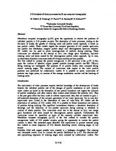
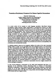
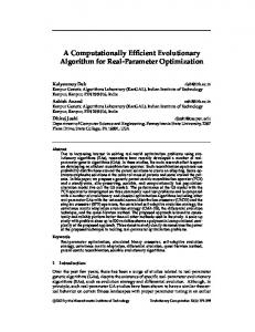
Fig. 2. Base resistance versus BE voltage for a 0:25 3 12:65 m HBT. Fig. 1. Total BE, BC, and CS capacitance: comparison between measurement (symbols) and HICUM (lines) for a 70-GHz BiCMOS SiGe process.

extracted from the basic capacitance equation (1) is the measured junction capacitance, is the applied where , , and are the zero-bias depletion junction voltage, and capacitance, built-in potential, and grading factor of the BE, BC, and CS junction. versus characterA linear regression of istic is applied to the transformation (2) as described in [4]. is chosen to maximize the magnitude of the linear correlation coefficient . For a single transistor extraction, the BC junction capacitance is split between the in, ternal and external transistor using the partitioning factor that is determined from Re at low current densities as suggested in [5]. Therefore, both internal and external built-in potential and grading factor of the BC capacitance are assumed to be identical. This method is preferred to the one described in [6], which is less sensitive to the junction capacitance measurement accuracy for small devices. Fig. 1 shows the results obtained for a device with an emitter m . Due to trench isolation, the area of bias dependence of the CS depletion capacitance is negligible to a very and hence turned off by setting the grading factor small value. B. Step 2: Junction Diodes The BE and BC junctions are described by two diodes, one for the ideal injection current and one for the recombination current, respectively. The CS junction is modeled by a classical diode equation. The extraction of the related parameters is done applying standard methods, i.e., linear regression of the logarithm of the junction currents. C. Step 3: Transfer Current at Low Injection and The low injection transfer current parameters , are extracted using the standard SGPM extraction routines: for and the forward Gummel-plot at V is

used, for the reverse Gummel plot at V and for the output conductance. The high-injection parameters and can be optimized for the forward and reverse current, respectively. D. Step 4: Series Resistances The series resistance is deduced from the inverse of transconductance versus the characteristics [7], is determined by while the extrinsic collector resistance characteristics in hard an optimization of the saturation. This parameter can be verified using the maximum oscillation frequency characteristics. The most recommended way for extracting the internal base resistance is the use of tetrode test structures [8]. If this test structure is not available, the modified input impedance circle method [9] can be applied. The drawback of the impedance circle method is its inaccuracy at low bias range. In Fig. 2 reusing this method are shown. sults for In the medium and high bias range the base resistance behavior can be simplified to (3) Either a nonlinear optimization or the following direct method V, can be applied for the parameter extraction. For and (3) can be rewritten as (4) as a function of the variable Plotting the determined gives a straight line with an appropriate value. The correct value is found when the correlation coefficient for the straight line is highest. Slope and -axes and , respectively. Choosing a point from intercept give V permits a direct calculation of the parameter a curve . E. Step 5: Avalanche Current For the extraction of the avalanche parameters, a forward output curve at low injection and constant is used. The avalanche current is described by [1, eq. (34)]. The collector current can be expressed as (5)

FRÉGONÈSE et al.: COMPUTATIONALLY EFFICIENT PHYSICS-BASED MODEL FOR CIRCUIT DESIGN – PART II

Fig. 3.

I and M versus V

at constant V

voltage.

Fig. 5.

1=(2f ) versus 1=J

289

for different CE voltages.

at a measurement frequency beyond the 3-dB corner frequency of the small-signal current gain . The next step consists from [10]. The of the determination of the transit time reads forward transit time

(10) with

Fig. 4. Linear regression for (8) with ). 1)C

x

=

C

and

y

= ln((M

0

The total collector current is combined by the avalanche free collector current and the multiplication factor . The can be directly determined by measuring avalanche current the decrease of the base current (6) V . Comwith respect to the base current bining (5) with (6) the multiplication factor can be determined

and where is the total base–collector junction capacitance. The standard method consists of a first-order approximation in fitting the low-current part of the curve in Fig. 5 with a straight line. The intercept with the axis allows the determination of as a function the low-current density value of the transit time of . The BC voltage can be calculated by , using the BE voltage where the fit above described is optimal. This of the method assumes a constant slope second term in (10). In [11], the limits of this standard method have been discussed in detail. It has been pointed out that the bias dependence and in particular the bias dependence of the transconductance has to be taken into account. Therefore, a taylor development of the second term of (10)

(7) (11) Fig. 3 shows as a function of with constant . The BC voltage dependence of the base current decrease can be observed as well as the resulting multiplication factor increase. Next, combining [1, eq. (34)] with (5) and reordering leads to (8)

is made. Using [1, eq. (33)], permits us to reorganize (11) (12) With (12), (10) can be rewritten

Using a simple linear regression, (8) permits the extraction of the avalanche parameters and (cf. Fig. 4) F. Step 6: Transit Time at Low Injection The transit time extraction method uses -parameter measurements at various collector current densities and various or . The transit frequency is determined using (9) Im

(13) , and . Now, from the plot versus the parameters , and can be optimized and the value of determined from . This modified extraction method minimizes the error curve and gives between (10) and the measured a very accurate low transit time. It has been verified by applying value is known. it to simulated data, where the with

290

Fig. 6. Low-current transit time


versus V

.

Fig. 6 shows the determined as a function of is described by BC voltage dependence of

. The

Fig. 7.

1

Fig. 8.

Critical current I

Fig. 9.

1

versus collector current I

and for different V

.

(14) with

and the parameter . The parameters and are determined and by a direct method, choosing two points and calculating (15) versus collector–emitter voltage.

(16)

G. Step 7: Critical Current The high-current transit time parameters are determined by . is defined as analyzing the curves (17) and for an investigated technology shown in Fig. 7. The increase of the transit time at high current densities is modeled by [1, eq. (2)] (18) that depends only on Inspecting the detailed [1, eq. (2)] gives with . Plotthe normalized variable versus should give only one curve inting . The first step consists of the determination dependent of of the appropriate values by using an iterative method. For , we get the same value for each . by This property determines an initial guess for value. It can be graphically interchoosing an initial preted as the intercepts of a horizontal line ( ) with curves (see Fig. 7). the versus the variable Next, the curves are plotted. As pointed out before, these curves should be superimposed. The iteration process is repeated by shifting the horizontal line until the superposition is optimized. From a practical point of view, the range of interest (to accurately determine the ) is near . Fig. 8 shows the resulting

versus normalized current I =I

for different V

.

characteristic with its influencing model parameters , , and . The parameters can be determined using a nonlinear optimization routine with the complete model equation given in [1]. H. Step 8: Transit Time at High Injection and , and can be extracted The parameters versus curve (Fig. 9). In the medium and from the can be neglected comhigh current region the influence of pared to . The resulting behavior is described by the first term of [1, eq. (2)]. Choosing from Fig. 9 two specific points at and , one can calculate at at

(19) (20)


Fig. 10.

Normalized I

=I

versus V

for different V

(0.7, 0.8, 0.9 V).

291

Fig. 12. Output characteristics for high current densities for a 0:25 3 12:65 m HBT on a 70 GHz STMicroelectronics technology.

Fig. 11. Comparison of the normalized high-current correction charge as a function of V .

Dividing (19) by (20) one can write

Fig. 13.

(0:5; 0;

(21) A simple analytical solution for does not exist. Numerically it can be calculated using conventional algorithms to determine zeros for a given function like bisection algorithm. Finally (19) can be rearranged to calculate

(22) The parameters and can be extracted from the low curversus ( ). Calcurent part of the curve lation of [[1, eq. (2)]] with and rewriting (18) gives the emitter portion of transit time increase

DC current gain for a 0:25 3 12:65 m HBT transistor at V

00:5) V; (70 GHz, STMicroelectronics).

=

I. Step 9: Temperature Parameters is extracted by global optimization The thermal resistance V versus curves at of normalized different constant values at room temperature. Different are presented in Fig. 10. For the lowest normalized value, there is no self-heating. We can observe the effect of the avalanche phenomenon at high reverse bias (cf. Step V, the self-heating makes increase at 2). At low bias, until the avalanche phenomenon takes over. Finally, , the self-heating is predominant and increases at highest , masking the avalanche phenomenon. The temperature dependence related model parameters are determined using standard methods. J. Step 10: Transfer Current at High Injection

(23) Application of a linear regression to

The normalized high-current correction charge is given in [1, eq. (29)]. Two parameters, and , have to be extracted and to model this correction. The normalized charges , can be calculated using the relevant relations [1] as a thus, function of the internal BE and BC voltages and temperature

(24) allows the direct determination of

and

.

(25)

292


Fig. 14. Transit frequency versus collector current for a 0:25 3 12:65 m HBT at V = ( 0:5; 0:25; 0; 0:25; 0:5; 1; 1:5) V; (70 GHz, STMicroelectronics).

0

0

Fig. 17.

Transconductance

(0:47; 1:7; 4:6; 8:9) mA and

GHz, STMicroelectronics).

y V

and input conductance y for I = = 0 V for a 0:13 3:53 m HBT; (230

3

Transit frequency versus collector current at V = V for a 0:13 3:53 m HBT; (230 GHz, STMicroelectronics).

Fig. 15. (

00:5; 00:25; 0; 0:25; 0:5)

Fig. 16. (

3

Unilateral gain versus collector current

I

at

00:5; 00:25; 0; 0:25; 0:5) V at 20 GHz for a 0:13 3 3:53 m

V

Fig. 18. Forward Gummel plot, V

= 0 V; (70 GHz, Infineon).

Fig.

forced

=

HBT; (230

GHz, STMicroelectronics).

The resulting characteristic in Fig. 11 can be fitted using the and nonlinear optimization or choosing two points and calculating the model parameters analytically

Here, (26)

(27)

19. Output

curves

with

(4; 7; 12; 20; 31; 46) A; (70 GHz, Infineon).

base

current,

I

=

is the normalized injection width and is the low-injection transfer current [2] at the respective terminal voltages. Fig. 11 compares model and measurements of the normalized high current correction charge. Fig. 12 shows the output characteristics for high current densities where this effect is particularly pronounced.


293

B. 230-GHz SiGe Technology of STMicroelectronics [14] Parameters for a HBT with emitter dimensions of 0.3 3.7 m of an advanced BiCMOS technology [14] have been extracted (see Figs. 15–17). C. 70-GHz SiGe Technology of Infineon [15] Model playbacks for a 0.25 10.15 m device in CBEBC configuration of a SiGe-technology [15] with copper metallization and a selective epitaxy are presented (see Figs. 18–20). D. 90-GHz SiGe-LEC Technology of Atmel [16] Fig. 20. Transit frequency, V Infineon).

= (0:375; 0:5; 0:75; 1:0; 2:0) V; (70 GHz,

A 0.5 9.9 m device of a low-emitter concentration (“real”) HBT technology [16] has been investigated (see Figs. 21–22). IV. CONCLUSION A step-by-step extraction methodology for the most important model parameters of the new compact bipolar transistor model HICUM/L0 was presented (see [2]). The methodology was applied to data from different technologies. Presented results showed good agreement with the data and emphasized the suitability of HICUM/L0 to describe bipolar transistors with sufficient accuracy for most applications. REFERENCES

Fig. 21.

Fig. 22.

Forward Gummel plot at V

= (0:3; 0:8; 1:8) V; (90 GHz, Atmel).

Transit frequency versus collector current density for

V

=

(0:3; 0:5; 0:8; 1:2; 1:5; 1:8) V; (90 GHz, Atmel).

III. EXPERIMENTAL RESULTS HICUM/L0 parameters have been extracted for several different technologies besides that presented earlier in [12]. A. 70-GHz SiGe Technology of STMicroelectronics [13] Results of the application of the previous described methods for a 70-Ghz technology [13] are shown in Figs. 12–14.

[1] M. Schroter, S. Lehmann, S. Fregonese, and T. Zimmer, “A computationally efficient physics-based compact bipolar transistor model for circuit design —Part I: Model formulation,” IEEE Trans. Electron Devices, vol. 53, no. 2, pp. 279–286, Feb. 2006. [2] S. Lehmann and M. Schroter. (2005) HICUM/Level0. [Online]. Available: http://www.iee.et.tu-dresden.de/iee/eb [3] M. Schroter, H.-M. Rein, W. Rabe, R. Reimann, H.-J. Wassener, and A. Koldehoff, “Physics- and process-based bipolar transistor modeling for integrated circuit design,” IEEE J. Solid-State Circuits, vol. 34, no. 11, pp. 1136–1149, Nov. 1999. [4] D. Berger, D. Celi., M. Schroter, M. Malorny, T. Zimmer, and B. Ardouin, “HICUM parameter extraction methodology for a single transistor geometry,” in Proc. IEEE BCTM, Monterey, CA, 2002, pp. 116–119. [5] D. Berger, N. Gambetta, D. Celi, and C. Dufaza, “Extraction of the BC capacitance splitting along the base resistance using HF measurements,” in Proc. IEEE BCTM, 2000, pp. 180–183. [6] B. Ardouin, T. Zimmer, H. Mnif, and P. Fouillat, “Direct method for bipolar BE and BC capacitance splitting using high frequency measurements,” in Proc. IEEE BCTM, Minneapolis, MN, 2001, pp. 114–117. [7] D. Berger and D. Celi, “HICUM parameter extraction methodology for a single transistor geometry,” presented at the Proc. Second Eur. HICUM Workshop, Dresden, Germany, Jun. 2002. [8] H.-M. Rein and M. Schröter, “Experimental determination of the internal base sheet resistance of bipolar transistors under forward-bias conditions,” Solid State Electron., vol. 34, pp. 301–308, 1991. [9] T. Nakadai and K. Hashimoto, “Measuring the base resistance of bipolar transistors,” in Proc. IEEE BCTM, Minneapolis, MN, 1991, pp. 200–203. [10] B. Ardouin, T. Zimmer, D. Berger, D. Celi, H. Mnif, T. Burdeau, and P. Fouillat., “Transit time parameter extraction for the HICUM bipolar compact model,” in Proc. IEEE BCTM, Minneapolis, MN, 2001, pp. 106–109. [11] M. Malorny, M. Schröter, D. Céli, and D. Berger, “An improved method for determining the transit time of Si/SiGe bipolar transistors,” in Proc. IEEE BCTM, 2003, pp. 229–232. [12] M. Schroter, S. Lehmann, H. Jiang, and S. Komarow, “HICUM/Level0 – A simplified compact bipolar transistor model,” in Proc. IEEE BCTM, 2002, pp. 112–115.

294


[13] H. Baudry, B. Szelag, F. Deliglise, M. Laurens, J. Mourier, F. Saguin, G. Troillard, A. Chantre, and A. Monroy., “High performance 0.25 m SiGe and SiGe:C HBT’s using non selective epitaxy,” in Proc. IEEE BCTM, Minneapolis, MN, 2001, pp. 52–55. [14] P. Chevalier, C. Fellous, L. Ruhaldol, D. Dutartre, M. Laurens, T. Jagueneaul, F. Leverdl, S. Bord, C. Richar’, D. Lenoble, J. Bonnouvrier, M. Martyl, A. Perrotin, D. Gloria, F. Saguin, B. Barbalat, R. Beerken, N. Zerounian, F. Anie, and A. Chantre, “230 GHz self-aligned SiGeC HBT for 90 nm BiCMOS technlogy,” in Proc. IEEE BCTM, 2004, pp. 225–228. [15] W. Klein and B.-U. H. Klepser, “75 GHz bipolar production technology for the 21st century,” in Proc. Eur. Solid-State Device Res. Conf., Leuven, Belgium, 1999, pp. 88–94. [16] J. Berutgen, A. Schueppen, P. Maier, M. Tortschanoff, W. Kraus, and M. Averweg, “SiGe technology bears fruits,” Mater. Sci. Eng.: B, vol. 89, no. 1, pp. 13–20(8), Feb. 2002.

Sébastien Frégonèse was born in Bordeaux, France, in 1979. He received the M.Sc. and Ph.D. degrees in electronics from the University of Bordeaux, in 2002 and 2005, respectively. During his Ph.D. work, he investigated bulk and thin SOI SiGe HBTs, with emphasis on compact modeling. He has recently joined the Technical University of Delft, the Netherlands, where his research activities deal with FET emerging devices, focusing on process and device simulation.

Steffen Lehmann was born in Hoyerswerda, Germany, in 1974. He received the M.S. degree in electrical engineering from the Technical University Dresden, Dresden, Germany, in 2004, working on parameter extraction for the HICUM bipolar compact model and high frequency on-wafer measurements. He is currently pursuing the Ph.D. degree at the same university, investigating advanced SiGe processes, focusing on device simulation and compact model development.

Thomas Zimmer was born in Wollbach, Germany. He received the M. Sc. degree in physics from the University of Würzburg, Würzburg, Germany, in 1989 and the Ph. D. degree in electronics from the University of Bordeaux, France, in 1992. Since 2003, he has been a Professor at the University of Bordeaux, France. His research focuses on characterization and modeling of high-frequency devices, in particular Si/SiGe heterojunction bipolar transistors. He is co-founder of the company XMOD Technologies and he has published about 100 technical papers related to his research.

Michael Schroter received the Dipl.-Ing. and Dr.-Ing. degrees in electrical engineering and the “venia legendi” on semiconductor devices in 1982, 1988, and 1994, respectively, from the Ruhr-University Bochum (RUB), Bochum, Germany. From 1993 to 1996, he was with Nortel and Bell Northern Research, Ottawa ON, Canada, first as Senior Member of Scientific Staff and later as Team Leader and Advisor, continuing the bipolar transistor modeling and parameter extraction activities. During 1994 to 1996, he was also Adjunct Professor at Carleton University, Ottawa. In 1996, he joined Rockwell Semiconductor Systems, Newport Beach, CA, as a Group Leader, where he established the RF Device Modeling Group and was responsible for modeling (Si, SiGe, AlGaAs) bipolar transistors, MOS transistors and integrated passive devices with emphasis on high-frequency process technologies and applications. In 1999, he was appointed Full Professor as the Chair for Electron Devices and Integrated Circuits at Dresden University of Technology, Dreseden, Germany. In 2003, he was also appointed Research Professor (part-time) at the University of California at San Diego. He has published several book chapters and is the author or coauthor of more than 80 technical publications. He also has given numerous lectures and invited tutorials on compact device modeling at international conferences and industrial sites, and is a regular reviewer for internationally renowned scientific journals. He is the author of the compact bipolar transistor model HICUM which has become an industry-wide standard. He is a cofounder of XMOD Technologies, a start-up company specializing in high-frequency semiconductor device modeling services for foundries and design houses. He is also on the Technical Advisory Board of RFMagic, a communications circuit design company in San Diego, CA. Dr. Schroter was a member of the BCTM CAD/Modeling subcommittee from 1994 to 2001, which he chaired from 1998 to 2000.

Didier Celi was born in Suresnes, France, in 1956. He received the degree from Ecole Superieure d’Electricite in 1981. In 1982, he joined the semiconductor division of Thomson-CSF, then the Central R&D of SGS-Thomson Microelectronics, now STMicroelectronics, Crolles, France. He has worked in the field of modeling for advanced bipolar and BiCMOS technologies, including model development, parameter measurement, and extraction tools. Presently, he is responsible for BiCMOS device modeling as Project Manager

Bertrand Ardouin received the M.S. and Ph. D. degrees in electrical engineering from the University of Bordeaux 1, France, in 1998 and 2001 respectively. His research activities were SiGe HBTs advanced modeling and characterization, with special focus on parameter extraction for the HiCUM bipolar compact model and high frequency on-wafer measurements. In 2002, he has been one of the co-founders of Xmod Technologies, Talence, France, a startup company working in the modeling field, where he is now R & D director. His main work is development of parameter extraction software for advanced compact models and modeling activities for various BiCMOS SiGe processes.

Helene Beckrich was born in Thionville, France, on August 7, 1979. She received the M.Sc. degree in physics from the Ecole Nationale Superieure de Physique de Strasbourg in 2002, after which she joined STMicroelectronics, Crolles, France, where she is currently pursuing the Ph.D. degree. Her research interests are modeling of RF power transistor in Silicon with emphasis on modeling of thermal effects and investigation of electrothermal interaction between semiconductor devices.


Pietro Brenner was born in Dillingen, Germany in 1965. He received the M.S. degree in physics from the Technical University Munich, Munich, Germany, in 1993. From 1994 to 1996 he was a Research Assistant at the Fraunhofer Institute for Atmospheric Environmental Research (IFU), Garmisch-Partenkirchen, Germany, where he was working on the development of a mobile Lidar ozone and aerosol measurement system. In 1996 he joined Siemens Semiconductors, now Infineon Technologies, where he has been working for seven years on characterization and modeling of Infineon’s RF-BiCMOS technologies. His general research interest lies in modeling and characterization of semiconductor devices and circuits. Main focus was the development of geometry-scaleable RF-device models for integrated passive devices and SiGe-Transistor modeling. A secondary field has been the development of enhanced test structures for fast on-wafer characterization and improvement of parameter extraction methodology. In 2003 he moved to the analog design methodology where he is currently working on behavioral modeling and simulation methodology. Now, his main focus is the development of application-specific behavioral models and model-based simulation methodology for analog-, RF- and mixed-signal design.

295

Wolfgang Kraus (M’83–SM’01) received the M.S. and Ph.D. degrees in electrical engineering from the University of Saarland, Saarbrücken, Germany, in 1982 and 1988. During his M.S. thesis he worked on parameter extraction for BJT’s, and his Ph.D. thesis was on numerical methods for RF-noise modeling of semiconductor devices. From 1982 to 1984 he did integrated circuit design for Philips, Nuremberg, and BOSCH, Reutlingen, both in Germany. From 1988 to present he is with Atmel Germany GmbH, Heilbronn Germany, formally TEMIC, having worked in the areas of integrated circuit design, CAD, and presently working in the area of modeling for circuit design. During the time of his CAD activities he was one of the main contributors to a mixed-signal simulator built on top of ELDO from ANACAD/Mentor Graphics. Dr. Kraus is a member of VDE, Representative of Atmel on the Compact Model Council, and a member of the modeling subcommittee of the BCTM since 2004.

A Computationally Efficient Physics-Based Compact ... - TU Dresden IEE

A Computationally Efficient Physics-Based Compact ... - TU Dresden IEE

Suggest Documents