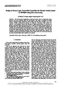
A COMPUTER SIMULATION OF TUNED PID AND CONTINUOUS SLIDING MODE FES CONTROL S. Jezernik*, R. Riener** *Aalborg University, Center for Sensory-Motor Interaction, Fredrik Bajersvej 7D3, 9220 Aalborg, Denmark, e-mail:
[email protected] **Technical University of Munich, Inst. of Automatic Control Eng. (LSR), Arcisstr. 21, 80333 Munich, Germany, e-mail:
[email protected] Abstract Functional Electrical Stimulation can restore movement in certain paralyzed individuals. Electric current pulses excite the intact peripheral nerves, cause the muscles to contract and generate joint movements. Since this physiological and biomechanical system is highly nonlinear and time-varying, feedback control is necessary for satisfactory FES control of the joint angles. In this study, a continuous computer model of a human knee was developed, and was used to compare the performance of widely used PID controller, with a newly developed sliding mode control strategy. Both strategies did compensate for the muscle fatigue effect, but the reference knee angle trajectory tracking of the tuned PID controller was poor compared to the sliding mode controller. The simulation results confirm that the sliding mode control might prove a very good candidate for precise trajectory tracking of the FES induced movements. Introduction Functional Electrical Stimulation (FES) can be used to restore movement to paralyzed extremities in e.g. spinal cord injured people. In FES, artificially generated electric fields excite intact nerves innervating paralyzed muscles to produce muscle contractions, and thus joint movements. To restore lost functionality (e.g. walking, hand movements) FES has to be appropriately controlled. Control output variables are either stimulation frequency, amplitude or stimulus pulsewidth. A possible control strategy is to control the position (angles) of the joints for the desired task, mimicking natural central nervous system (CNS) control. Control of joint angles by FES is non-trivial because of muscle fatigue and nonlinearities in muscle activation, muscle dynamics and biomechanics. Time-variance, parameter variations and nonlinearities of the plant result in poor open-loop control performance, necessitating feedback control [1], which is inherently present during CNS control. Two closed-loop strategies were compared in the present study: tuned PID control and continuous approximate sliding mode (SM) control. The latter was previously shown to possess some inherent adaptation, guarantees closed-loop stability, and requires little knowledge of the plant model [2]. Control strategies were tested on a computer model of the human knee. Plant model input was the stimulation pulse width and the plant output was the knee joint angle. Stimulation frequency and current amplitude were kept constant. Only one knee extensor muscle group was stimulated in this study. Methods Plant model: The biomechanical model of the human knee of a siting individual includes muscle activation, muscle contraction dynamics and segmental dynamics [3]. The muscle activation block models nerve fiber recruitment, spatial and temporal summation effects, and frequency dependent muscle fatigue. Muscle activation depends on intracellular Ca++ ion concentration. Muscle fatigue effect can be switched on or off. The muscle contraction dynamics block computes active knee joint torque produced by muscle contraction using force-length and force-velocity relations, and moment arm computations. Segmental dynamics block computes knee joint angle produced by sum of active and passive (knee damping, knee elasticity) knee joint torques. The resulting plant model is highly nonlinear and can be described by a system of 5 ordinary differential equations with state space vector x=[x1 x2 x3
x4 x5]T. x1 is the knee joint angle (0° corresponds to 90° knee flexion and 90° to full knee extension), x2 is the knee joint velocity, x3 is the muscle fitness (fatigue variable), x4 is the normalized Ca++ ion concentration and x5 is the derivative of the normalized Ca++ ion concentration. Chosen model parameters represent a generic (average) person and have been adapted to experimental data from literature and to own identification/model-validation experiments. PID controller: was tuned by Ziegler-Nicholes relay experiment procedure [4]. The system was forced to exhibit limit-cycle oscillations and the ultimate oscillation period and amplitude were determined. PID parameters were computed from the latter according to Ziegler-Nicholes rule of thumb, which provides good closed-loop performance. Sliding mode controller: Sliding mode control can be applied to control systems that are affine in control input and thus have a general form:
x& (t ) = f ( x, t ) + B( x, t ) ⋅ u(t ) where B is a nxm input matrix. Control signal u(t) is computed in such a way that the closed system reaches a predefined submanifold S={x: s(x)≡0} and afterwards remains on that submanifold. Control u(t) required for the system to remain on the submanifold (sliding mode) is called equivalent control ueq(t). The submanifold is chosen to be an intersection of hyperplanes: s(x)=K*(xr-x)≡0, where x represents the state space vector, xr the reference vector and K is a constant mxn matrix. Equivalent control can be computed from the requirement ds/dt=0, meaning that after the submanifold is reached, the system remains on it. • u eq = ( KB ) −1 − K ⋅ f ( x, t ) + K ⋅ x r (t )
The submanifold reaching condition and stability of the sliding mode are guaranteed by the Lyapunov method. Choose the Lyapunov function candidate as
V = sT s which is a positive definite function. Its time derivative is then: •
•
V = 2sT s
The discontinuous SM control law that makes dV/dt negative definite is: ds/dt=-D*sign(s). Since this discontinuous law introduces chattering, a better choice is a continuous SM control: ds/dt= -D*s, where D is a positive definite matrix. s will thus eventually asymptotically approach zero. Using a relation s=K*(xr-x) the following control law can be derived: •
u(t ) = ( KB ) −1 [ K x r − Kf ( x, t ) + Ds( x )] = u eq + ( KB ) −1 Ds( x )
Using a small enough sampling time Ts and assuming continuity of u(t), the following approximation can be used to derive approximate continuous SM control u(t): •
x (t ) ≈ f ( x (t ), t ) + B ( x (t ), t ) ⋅ u (t − Ts ),
Ts → 0
•
u(t ) = u(t − Ts ) + ( KB ) −1 [ s + Ds ]
s is chosen as s=Kp(x1r-x1)+Kd(x2r-x2)+Kf(x3r-x3)+Kg(x4r-x4)+Kdg(x5r-x5), where xir are the reference values and Ki are constants (controller parameters that were chosen to yield the best performance). Note that because we only have one input, s is a scalar and not a vector. Since Kf was set to zero, x3f did not need to be specified. The problem remained how to calculate the reference for concentration of Ca++ ions (x4r). Since a bigger knee angle requires larger pulse width of stimulation, and thus increased Ca++ ion concentration, the latter was scaled proportionally to the reference knee angle. System performance was not satisfactory, so a trick was used to improve it. The reference x4r was upregulated/downregulated with the hard-limited PI controlled knee angle error e1=x1r-x1. Positive e1
caused reference x4r to increase, and thus achieved the higher muscle activation needed to compensate for e1. Computer simulation: Simulations were performed in MATLAB/SIMULINK using simulation times 0.01 s for PID controller and 0.001 s for SM control. All state space variables were sampled at 0.01 s. Squarewave, ramp and sinusoidal reference tracking of the knee joint angle were evaluated. Results
o
Knee angle [o]
Knee angle [ ]
Figs. 1a and 1b show positive and negative knee angle step responses of model controlled by PID (dashed line) and SM controller (solid line). Table 1 summarizes and compares the results. The SM
T [in 10 ms]
T [in 10 ms]
Fig.1a
Fig. 1b
controller outperforms the PID controller in all performance measures. Table 1: Measurements of step response parameters
PID pos. step SM pos. step PID neg. step SM neg. step
Dead Time Max. Over/Undershoot Td 0.08 s 14% 0.05 s 1.7% 0.07 s 31.6% 0.05 s 1.9%
5% Settling Time
10-90% Rise Time
1.45 s 0.54 s >3.00 s 0.39 s
0.37 s 0.36 s 0.25 s 0.20 s
o
Knee angle [ ]
o
Knee angle [ ]
Pulse width [µs]
Pulse width [µs]
Figs. 2a and 2b show square-wave tracking with period of 6 s over 40 s. The upper traces show controller output u(t) and the lower traces the knee joint angle. Again SM control achieves better tracking (integral of absolute error over second period: SMerror-integral=12.80os and PIDerror-integral=22.47os). Over 6 s the average absolute error was 2.13o for SM and 3.74o for PID controller, i.e. 1.60o more. SM reached steady-state errors smaller than 0.0001° two seconds after the step. Performance of both controllers deteriorated after 30 s, when the control signal started to saturate at 500 µs pulse width due to the effect of fatigue. SM tracking remained slightly better.
T [s]
F ig. 2a
T [s]
Fig. 2b
T [s]
Fig. 3a
Pulse width [µs] T [s]
Knee angle [o]
o
o
Knee angle [ ]
Knee angle [ ]
Pulse width [µs]
Pulse width [µs]
Positive and negative ramp tracking (period T=10 s) with fatigue switched off is shown in Figs. 3a and 3b and with fatigue switched on in Fig. 3c (SM: dashed line; PID: solid line). Saturation level for nerve fiber
Fig. 3b T [s]
Fig. 3c
recruitment was set to 800 µs instead of 500 µs as before. 500 µs pulse width saturation gave comparable results. Tracking error of SM controller was about 10 times smaller than that of PID (