equal to 1.5 umf for the whole width of the bed (umf = 1.8 [m/s]). ... coefficient of restitution, [-]. 100.0. 200.0. 300.0. 400.0. 500.0. 600.0. R. M. S. , [P a. ] 0.00. 0.10.
World Congress on Particle Technology 3
213 THE INFLUENCE OF PARTICLE PROPERTIES ON PRESSURE SIGNALS IN DENSE GAS-FLUIDISED BEDS: A COMPUTER SIMULATION STUDY B.P.B. Hoomans, J.A.M. Kuipers and W.P.M. van Swaaij Department of Chemical Engineering, Twente University of Technology, P.O. Box 217, 7500 AE Enschede, The Netherlands A hard-sphere discrete particle model of a gas-fluidised bed was used in order to study the influence of particle properties on pressure signals in dense gasfluidised beds. In the model the gas-phase hydrodynamics is described by the spatially averaged Navier-Stokes equations for two-phase flow. For each solid particle the Newtonian equations of motion are solved taking into account the inter-particle and particle-wall collisions. Pressure fluctuations inside the bed are strongly affected by the coefficients of restitution and friction: the more energy is dissipated in collisions the stronger the fluctuations are. The root mean square of the pressure fluctuations showed an almost linear dependency on the amount of energy dissipated in collisions during the simulation. Keywords: fluidisation, granular dynamics, computer simulation, discrete particle, collision properties.
INTRODUCTION With increasing computer power discrete particle models have become a very useful and versatile research tool to study the dynamics of dense gas-particle flows. In these models the Newtonian equations of motion are solved for each individual granular particle in the system. The mutual interactions between particles and the interaction between particles and walls are taken into account directly. Applications of this type of models are very diverse ranging from agglomerate dynamics (Thornton et al.1) to hopper flow (Langston et al.2). In this paper the discrete particle method will be used to model gas-fluidised beds. In fluidisation simulations the discrete particle models have a clear advantage over continuum models since the particle interactions are taken into account directly and consequently the necessity to specify closure relations for the solids-phase stress tensor, as encountered in continuum models (Kuipers et al.3 among many others), is circumvented.
Page 1
World Congress on Particle Technology 3 Tsuji et al.4 developed a soft-sphere discrete particle model of a fluidised bed based on the work of Cundall and Strack5. In this approach the particles are allowed to overlap slightly and this overlap is subsequently used to calculate the contact forces. Hoomans et al.6 used a hard-sphere approach in their discrete particle model of a fluidised bed which implies that the particles interact through binary, instantaneous, inelastic collisions with friction. Xu and Yu7 used a soft-sphere model similar to the one used by Tsuji et al.4 in their fluidised bed simulations but they also employed techniques from hard-sphere simulations in order to determine the instant when the particles first come into contact precisely. In static simulations the soft-sphere model has a clear advantage over the hardsphere model since it allows for multiple particle contact. The hard-sphere model requires a period of free flight in between collisions and is therefore not suited for static simulations. In fluidised beds however the particles are constantly in motion and here the hard-sphere model offers some advantages over the soft-sphere model. Firstly the hardsphere model has lower computational cost and secondly the mutual interactions between particles is determined analytically and not numerically like in the soft-sphere case. Hoomans et al.6 have shown that the dynamics of a fluidised bed depends strongly on the particle interaction parameters (i.e. coefficients of restitution (e) and friction (µ)). In the case where no energy is dissipated (i.e. e = 1 and µ = 0) no bubble or slug formation was observed and the bed showed a rather homogeneous fluidisation behaviour, whereas in the case where the impact parameters were given more realistic values (i.e. e = 0.9 and µ = 0.3) and hence energy is dissipated in collisions, bubble formation was observed and the bed behaviour appeared to be in much better agreement with that observed in reality. In this paper this dependency is investigated in more detail using the hard-sphere model.
HARD-SPHERE GRANULAR DYNAMICS Since most details of the model are presented in a previous paper6, the key features will be summarised briefly here. The collision model as originally developed by Wang and Mason,8 is used to describe a binary, instantaneous, inelastic collision with friction. The key parameters of the model are the coefficient of restitution (0 ≤ e ≤ 1) and the coefficient of friction (µ ≥ 0). Foerster et al.9 have shown that a third coefficient (coefficient of tangential restitution) should be used in order to describe the collision dynamics more accurately. This coefficient was implicitly assumed to be equal to zero in this work. In the hard-sphere approach a sequence of binary collisions is processed. This implies that a collision list is compiled in which for each particle a collision partner and a corresponding collision time is stored. A constant time step is used to take the external forces into account and within this time step the prevailing collisions are processed sequentially. In order to reduce the required CPU time neighbour lists are used. For each particle a list of neighbouring particles is stored and only for the particles in this list a check for possible collisions is performed.
EXTERNAL FORCES The incorporation of external forces differs somewhat from the approached followed in our previous paper6. In this work we use the external forces in accordance with those Page 2
World Congress on Particle Technology 3 implemented in the two-fluid model described by Kuipers et al.3 where, of course, the forces now act on a single particle:
(1) where mp represents the mass of a particle, vp its velocity, u the local gas velocity and Vp the volume of a particle. In equation (1) the first term is due to gravity and the third term is the force due to the pressure gradient. The second term is due to the drag force where β represents an interphase momentum exchange coefficient as it usually appears in twofluid models. For low void fractions (ε < 0.80) β is obtained from the well-known Ergun equation:
(2) where dp represents the particle diameter, µg the viscosity of the gas and ρg the density of the gas. For high void fractions (ε ≥ 0.80) the following expression for the interphase momentum transfer coefficient has been used which is basically the correlation presented by Wen and Yu10 who extended the work of Richardson and Zaki11:
(3) The drag coefficient Cd is a function of the particle Reynolds number and given by:
,
(4)
where the particle Reynolds number in this case is defined as follows:
(5)
GAS PHASE HYDRODYNAMICS The motion of the gas-phase is calculated from the following set of equations which can be seen as a generalised form of the spatially averaged Navier-Stokes equations for a two-phase gas-solid mixture. Continuity equation gas phase:
Page 3
World Congress on Particle Technology 3
. (6) Momentum equation gas phase:
.
(7)
In this work transient, two-dimensional, isothermal (T = 293 K) flow of air at atmospheric conditions is considered. The constitutive equations can be found in Hoomans et al.6. There is one important modification with respect to our previous model and that deals with the way in which the two-way coupling between the gas-phase and the dispersed particles is established. In the present model the reaction force to the drag force exerted on a particle per unit of volume is fed back to the gas phase through the source term Sp [Nm-3]. A more detailed discussion on this approach can be found in Delnoij et al.12. In the present model only the second term in equation (1) is involved in the two-way coupling.
RESULTS A number of simulations was performed in order to investigate the influence of the collision properties on the bed dynamics. As a test system we used the same system that was used
Page 4
World Congress on Particle Technology 3
Figure 1, Snapshots of particle configurations for three simulations. Upper: e = 1, µ = 0, middle: e = 0.99, µ = 0, bottom: e = 0.9, µ = 0.3. Table 1 System parameter settings for all simulations Particles Bed shape spherical width 0.15 [m] diameter 4.0 [mm] height 0.50 [m] material aluminium number of x-cells 15 density 2700 [kg/m3] number of y-cells 25 number 2400
Page 5
World Congress on Particle Technology 3 before by Tsuji et al.4, Hoomans et al.6 and Xu and Yu7. The most important system parameters are summarised in table 1. In all simulations the minimum fluidisation conditions were used as initial conditions while the values for the coefficients of restitution (e) and friction (µ) were varied. A time step of 10-4 seconds was used in all simulations and the gas inflow at the bottom was set equal to 1.5 umf for the whole width of the bed (umf = 1.8 [m/s]). The simulations were continued for 8 seconds real time and during the simulations the pressure in the bed 0.2 meter above the centre of the bottom plate was monitored. A typical run could be performed within 50 minutes of CPU-time on a Silicon Graphics Origin200 server (R10000 processor, 180 MHz). Snapshots of the particle configurations for three simulations are presented in figure 1. The two extreme cases (e = 1, µ = 0 (ideal) and e = 0.9, µ = 0.3 (non-ideal)) are shown there together with a simulation where e = 0.99 and µ = 0. In order to visualise the induced particle mixing during the fluidisation process, at t = 0 [s] a number of particle layers was marked by colour. It can be seen that in the ideal case barely any bubbles or slugs are being formed which enables the initial structure to remain intact for quite some time. In the non-ideal case the formation of bubbles and slugs can be observed clearly and due to these instabilities the particle mixing in the bed is much better. After 2 seconds the initial structure can still be observed in the ideal case whereas it has completely disappeared in the non-ideal case. The simulation with e = 0.99 resembles the ideal case very much although the particle mixing appears to be slightly better. This is a much more natural dependency than the one reported for instance by Hrenya and Sinclair13 using a two-fluid model which incorporates kinetic theory for granular flow in order to arrive at improved closure relations for the solids phase stress tensor where a change in e from 1.0 to 0.99 completely changed the hydrodynamic behaviour.
Figure 2, Pressure fluctuations at 0.2 [m] above the centre of the bottom plate. The computed pressure signals at 0.2 [m] above the centre of the bottom plate for the three simulations are presented in figure 2. It can be observed that the pressure fluctuations in the non-ideal case are much stronger than in the ideal case. In fact the pressure fluctuations turn out to depend strongly on the collision parameters. In figure 3 the root mean square (RMS) of the pressure signals is presented as a function of the coefficient of restitution.
Page 6
600.0
600.0
500.0
500.0
RMS, [Pa]
RMS, [Pa]
World Congress on Particle Technology 3
400.0
300.0
200.0
100.0 0.85
400.0
300.0
200.0
0.90 0.95 coefficient of restitution, [-]
Figure 3, Root Mean Square (RMS) of pressure fluctuations as a function of the coefficient of restitution.
100.0 0.00
0.10
0.20 0.30 coefficient of friction, [-]
0.40
Figure 4, RMS of pressure fluctuations as a function of the coefficient of friction.
It can clearly be observed that the RMS increases with decreasing value of the coefficient of restitution. The fact that, for instance, the RMS value for the simulation with e = 0.96 is higher than that for the simulation with e = 0.95 is due to the different dynamics which despite of the lower value for the coefficient of restitution causes a higher amount of energy to be dissipated in collisions during the simulation. With a slightly different initial condition this might change which is inherent of the complex (i.e. chaotic) nature of the system’s dynamics. In all the simulations which were performed in order to obtain the RMS values presented in figure 3, the coefficient of friction was set equal to zero. In the calculation of the RMS the initial stages of the simulation (approximately 2 [s]) were not taken into account in order to avoid start-up effects from influencing the results. In figure 4 the RMS is presented as a function of the value of the coefficient of friction. For all the simulations which were performed in order to obtain the RMS values presented in figure 4 the coefficient of restitution was set equal to 1.0. Here it can be observed that the RMS increases with increasing value for the coefficient of friction. In figure 4 the value for the RMS is lower for the simulation with µ = 0.25 than for the simulations with µ = 0.2 which is not expected. However the amount of energy dissipated in collisions for both simulations is not the same; in fact more energy is dissipated in the simulation with µ = 0.2 than in the simulation with µ = 0.25. In the latter case fewer collisions occurred and apparently the collisions that occurred had less impact. In figure 5 the RMS is plotted as a function of the energy dissipated in collisions during the entire simulation. All simulations performed in this study are included in this figure. It can be seen that the RMS increases almost linearly with the amount of energy dissipated in collisions in the system. For higher values of the dissipated energy (i.e. lower coefficients of restitution and/or higher coefficients of friction) the dynamics of the system becomes more complex which requires longer simulation times in order to obtain better statistics.
Page 7
World Congress on Particle Technology 3
600.0
RMS, [Pa]
500.0
400.0
300.0
200.0
100.0 0.0
0.5 1.0 dissipated energy, [J]
1.5
Figure 5, RMS of pressure fluctuations as a function of the energy dissipated in collisions during the simulation.
CONCLUSIONS A hard-sphere discrete particle model was used in order to investigate the effect of the collision parameters on the pressure signals inside a gas-fluidised bed. The bed dynamics is strongly affected by the values of the coefficients of restitution and friction. When ideal values (e = 1, µ = 0, i.e. no energy is dissipated in collisions) are specified nonrealistic dynamics is observed: no bubble or slug formation occurs and particle mixing is poor. When realistic values (e = 0.9, µ = 0.3) are specified bubble and slug formation are observed and the fluidisation behaviour is in much better accordance with that inferred from experimental observations. Pressure fluctuations inside the bed are much stronger than in the ideal case. With intermediate values for these coefficients the behaviour also changes gradually with pressure fluctuations becoming less strong when the coefficients are changed toward their ideal values. It turned out to be more convenient to determine the root mean square (RMS) of the pressure fluctuations as a function of the total amount of energy dissipated in collisions since this amount is affected by both the collision parameters and the system dynamics. The RMS values of the fluctuations show an almost linear increase with the amount of energy dissipated in collisions during a simulation. In the near future spectral analysis will be applied in order to investigate the pressure signals in more detail.
NOTATION Cd dp g
drag coefficient, [-] particle diameter, m gravitational acceleration, m/s2
Page 8
vp Vp
particle velocity vector, m/s particle volume, m3
World Congress on Particle Technology 3 mp p r Sp T t u
particle mass, kg pressure, Pa position vector, m momentum source term Eq. (7), N/m3 temperature, K time, s gas velocity vector, m/s
Greek symbols β ε µg τ ρg
defined in Eqs (2) and (3), kg/m3s void fraction, [-] gas viscosity, kg/ms gas-phase stress tensor, kg/ms2 gas density, kg/m3
REFERENCES 1
2
3 4 5 6
7
8 9 10 11 12
13
Page 9
Thornton, C., K. K. Yin, and M. J. Adams, 1996, Numerical simulation of the impact fracture and fragmentation of agglomerates, J, Phys. D: Appl. Phys. 29, 424. Langston, P. A., U. Tüzün and D. M. Heyes, 1995, Discrete element simulation of granular flow in 2D and 3D hoppers: dependence of discharge rate and wall stress on particle interactions, Chem. Engng Sci. 50, 967. Kuipers, J. A. M., K. J. van Duin, F. P. H. van Beckum and W. P. M. van Swaaij, 1992, A numerical model of gas-fluidized beds, Chem. Engng Sci., 47, 1913. Tsuji, Y., T. Kawaguchi, and T. Tanaka, 1993, Discrete particle simulation of two dimensional fluidized bed, Pow. Tech. 77, 79. Cundall P. A. and O. D. L. Strack, 1979, A discrete numerical model for granular assemblies, Géotechnique, 29, 47. Hoomans, B. P. B., J. A. M. Kuipers, W. J. Briels and W. P. M. van Swaaij, 1996, Discrete particle simulation of bubble and slug formation in a two-dimensional gas-fluidised bed: a hard-sphere approach, Chem. Engng Sci., 51, 99. Xu, B. H. and A. B. Yu, 1997, Numerical simulation of the gas-solid flow in a fluidized bed by combining discrete particle method with computational fluid dynamics, Chem. Engng Sci., 52, 2785. Wang Y. and M. T. Mason, 1992, Two-dimensional rigid-body collisions with friction, J. Appl. Mech., 59, 635. Foerster S. F., M. Y. Louge, H. Chang and K. Allia, 1994, Measurements of the collision properties of small spheres, Phys. Fluids, 6 (3), 1108. Wen, C. Y. and Y. H. Yu, 1966, Mechanics of fluidization, Chem. Eng. Prog. Symp. Ser., 62 (62), 100. Richardson, J. F. and W. N. Zaki, 1954, Sedimentation and fluidization: part I, Trans. Inst. Chem. Eng. 32, 35. Delnoij, E., F. A. Lammers, J. A. M. Kuipers and W. P. M. van Swaaij, 1997, Dynamic simulation of dispersed gas-liquid two-phase flow using a discrete bubble model, Chem. Engng Sci., 52, 1429. Hrenya, C. M. and J. L. Sinclair, 1997, Effects of particle-phase turbulence in gas-solid flows, AIChE J. 43, 853.