A conceptual framework for dynamic location-allocation analysis. E S Sheppard. University of Toronto, Department of Geography, Toronto, Ontario, Canada.
Environment and Planning A, 1974, volume 6, pages 547-564
A conceptual framework for dynamic location-allocation analysis
E S Sheppard University of Toronto, Department of Geography, Toronto, Ontario, Canada Received 28 June 1974
Abstract. To date, much of the work published on the problems of plant construction has been restricted to either determining the timing of the building, or forming static location-allocation models, with little attempt to combine the spatial and temporal aspects into one solution. By construction of a taxonomic tree, this paper demonstrates that the capacity expansion and the location-allocation solutions are just the simplest instances of a whole class of models. Formulation of these various possibilities is undertaken and it is shown that a fully integrated spatio-temporal plant-construction model can be derived, at least at the theoretical level. Although the derivations are in the form of deterministic programming models, the concluding section of the paper suggests possible ways in which these might be reformulated to allow for the fact that most planning takes place in an uncertain environment. 1 Introduction
The starting point of this paper was the review of location-allocation models developed by Scott (1971a). In that review it was evident that this literature has so far largely ignored two fundamental aspects of a dynamic location-allocation problem. These are first the effect, on the models, of demand patterns which change over time, and second the problem of when to build plants and how big to build them. A reading of the scant collection of relevant literature reveals that at present there exists on the one side static location-allocation models, and on the other a series of capacity-expansion models. The former find solutions to the optimal locations of plants under static conditions of demand, and the latter attack the problem of selecting the best timing and size for new factory construction with changing demand, but in a nonspatial world. Attempts to link these two approaches have on the whole been implicit rather than explicit, being oriented toward very specific problems (for example George, 1971). Erlenkotter (1967; 1969) is the only person to attempt to deal with the more general class of problems which exist. Because of this, the aim of this paper is to provide a more complete theoretical structure for the problem in order to illustrate explicitly the links between these two groups of models and to show the spatial aspects of the dynamic plant-construction problem. It should be noted in the following that specific techniques of solution of the particular problems have, in large, been neglected. Instead discussion is limited to general strategies under alternative assumptions about future variations in demand. The paper is constructed in the following way. First the conceptual framework— the variables involved in the problem and their effect on the solution—is discussed. Then a formal statement of the different possible models outlined in the conceptual framework is set up, with some discussion of the work done on these to date. Finally a brief summary of the possible planning strategies over time is outlined. >2 Development of a conceptual framework
First the general problem will be stated. It is desired to find optimal policies to determine the location, size, and timing of new plant construction or old plant expansion for a single-product firm in a world of changing demand. The variables of the problem may then be stated as factory size, time of construction, and factory
548
E S Sheppard
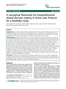
location. These represent the three basic dimensions, and alternative models of varying complexity may be outlined according to whether each variable is fixed a priori or to be determined in the solution. Ceteris paribus, each variable has a characteristic effect on the problem. Factory size is subject to economies of scale, the cost per unit being less for large plants than for small ones. Therefore to satisfy a given demand it would be preferable to build one plant, as large as is necessary. Location has an effect such that cost per unit rises with the distance each unit has to be moved, although this rise will probably be less than proportional to distance because of the structure of freight rates. As for the effect of timing, it is better to build later on, because of the fall in the value of money with time when discounted to present-day figures. Unfortunately these variables work against one another to the extent that there are three trade offs which must be considered. First there is the question of whether to build a large plant now, or to build a series of smaller ones, as they become required by demand, later on in the planning period. Thus one is trading off economies of scale under the former possibility versus a saving due to a fall in costs with time. The best strategy will depend on the size of scale economies possible relative to the interest rate (which determines the value of money in the future). Also one would need to consider variations in demand over time: whether it is growing or falling, and whether there is a heavy penalty for undersupplying customers. (If there were no such penalty then it would perhaps be cheaper to build one large plant in the last time period or, better still, not to build at all.) The second trade off is between scale economies and distance. To minimise the latter, ideally each consumer should have his own production plant, but this is very costly in terms of scale diseconomies. On the other hand one large plant, wherever it is located, may incur large transportation costs. Again the optimal solution will depend on the relative size of the two cost factors. Finally there is the relation between distance and timing. Here a conflict between the two factors will not necessarily occur, unlike the situation envisaged in the second trade off, as it may be possible to build both late and close to the market. The solution depends on the forecasted changes in the distribution of potential customers, and the effect of this relative to the effect of the interest rates on the model. Each of these trade offs gives only a partial solution to our problem. If all three factors are allowed to vary, then it becomes difficult to describe the intricacies of the problem in verbal terms. One possibility is to see it as a choice between building a large plant now with scale economies but high transportation costs, or to build a dispersed set of smaller plants later on, incurring diseconomies of scale but lower shipping costs. Thus even if economies of scale are so large in the former case as to outweigh discounted building costs for the smaller plants (implying construction of one large plant is optimal), when transport is considered it may be so costly for a single plant that a policy of dispersed plants becomes preferable. From a different angle, one might compare the possibility of building many smaller plants now, giving low transport costs in the future, as opposed to building one large plant sometime from now (that is with relatively cheaper building costs) with no costs up to that time but considerable (although discounted) transport costs subsequently. This by no means exhausts the possibilities that must be considered here, and it is evident that with three conflicting variables, each contributing its own distinct qualities to the solution, increased realism must be paid for by greater computational difficulty. The taxonomic tree (figure 1) is built based on these factors, allowing each in turn to be either fixed a priori or variable. For any particular operating policy this gives rise to one problem with nothing variable (with a trivial solution), plus three problems
•fl
ss
time fixed
plant size fixed
!
o
time fixed
;
o3
time variable (Manne, Kirby)
^f=r
time fixed
a.
time variable (Erlenkotter)
13 O
v- 3
o
s.§t
55*
tree fo £•*•
3
5* 5* o 3
o> a a
o
o PS
o* 3
1
time fixed
p O* R
O
II
time variable
T3 •« 2 .
Pi
o o 23 uroble
3 / ^» Pi s
ps 00
O
o
g:g\B time fixed
% s. 5*
» o*
g 8
time variable
o 3
h3
§•« 3 2* 0,
(2a)
J
(2b)
XtOcft-Siht) > 0 ,
* = 0,.., 7 \
(2c)
M\t > (Xft-stht),
t = 0,..-, T,
(2d)
\rA=l,0,
(2e)
st>0.
(2f)
This is solved for sif In equation (2a), Xit is unity if plant i has been built by time t, and zero otherwise; Xt is unity if there is undersupply of the product at time t, and zero at all other times; and S^max is the capacity needed to supply the largest demand occurring. Here a minimum of the accumulated costs of construction, undersupply, and production is sought over all time periods, subject to the constraints that once the plant is built it is in use ever after, equation (2b), and that a penalty is only applied when the product is undersupplied, not when it is oversupplied, equations (2c) and (2d). 3.2.4 Plant size and timing are both variable. Minimise f ' Stt max !~ T r
\TPtXft 0
T
+ ciQsKl+ir+
\_t=0
I
T
Pt(xft-stht)\t+
t = r+ l
I
ftisM dSi,
(3a)
t = r+i
subject to ht-ht-i
> 0 ,
\(xit-si\it)>0, MXt > (XJ, - Si Xit),
f'=0,...lr,
,
(2b)
t = 0,...,T,
(2c)
t = 0,..., T ,
(2d)
X,„Af = 1 , 0 ,
(2e)
st>0,
(2f)
0 < r < T.
(3b)
553
A conceptual framework for dynamic location-allocation analysis
Solution is for sf and r, a problem also discussed by Kirby (1971). He shows that, for st split into a finite number of intervals [namely the discrete version of equation (3a)] and with demand known at all times, a dynamic programming format may be used to determine the optimal policy of plant construction and possible subsequent expansion. Each new construction constitutes a stage in the dynamic programme, and within each stage all possible construction options are considered. The cheapest route to each such option is chosen, leading ultimately to the selection of the best sequence of all those that are feasible solutions to the problem. For the rest of this paper the term in ft(st) will be omitted for the sake of brevity. It will occur in all problems with variable timing or size of plant construction, and can be readily added in as needed. In addition, as noted earlier, the size of the plant may be expressed as a discrete or continuous variable. The discrete form will be turned to in the remainder of this exposition as it is more consistent with the mathematical programming type of format that the rest of the problem is expressed in. 3.3 The single-plant many-region policy Under this policy the construction or expansion of just one plant is to be optimised, although the existence of many regions introduces a spatial dimension to the supply side of the problem. 3.3.1 All three variables are fixed. This has a trivial solution. 3.3.2 Timing alone is variable. Minimise £
£ptXft
+ Ci(l + ir+
r =0/=l
I
Fin.
(4)
t = r+ l
This is solved for r (0 < r < T). The i^ /r 's are known, as both the xJt's and