A Conceptual Guide to Detection Probability for Point Counts and Other Count-based Survey Methods1 D. Archibald McCallum2 ________________________________________
Abstract
Introduction
Accurate and precise estimates of numbers of animals are vitally needed both to assess population status and to evaluate management decisions. Various methods exist for counting birds, but most of those used with territorial landbirds yield only indices, not true estimates of population size. The need for valid density estimates has spawned a number of models for estimating p, the ratio of birds detected to those present. Wildlife biologists can be assisted in evaluating these methods by appreciating several subtleties of p: (1) p depends upon the duration of the count, (2) p has two independent components, availability of cues and detectability of cues, (3) detectability is a function of both the conspicuousness of cues (e.g., vocalizations, conspicuous movements) and the abundance of cues, and (4) discontinuous production of cues lowers availability, which has a direct and sometimes profound effect on p. Two recently-updated methods of estimating p, doubleobserver sampling and distance-sampling, are better suited to estimating detectability, while two others, double sampling and removal sampling, are better suited to estimating availability. While none of the four offers a complete solution at present, hybrids are under development, and a technique that can yield estimates of availability and detectability from survey data may be available in the near future.
Unlike most fish, insects, and nocturnal mammals, birds are typically surveyed without capturing or marking individuals. A number of passive sampling techniques, e.g., spot-mapping, line transects, and point counts, are commonly used for estimating numbers of birds. A complete taxonomy of sampling and analytical methods is given by Thompson (2002). The accuracy and precision of most techniques currently used to count birds has been questioned, because of their failure to provide estimates of detection probability (Nichols et al. 2000, Bart and Earnst 2002, Farnsworth et al. 2002, Rosenstock et al. 2002, Thompson 2002).
Key words: abundance of cues, availability, bird survey, census, conspicuousness, detectability, detection probability, distance sampling, double sampling, double-observer sampling, index ratio, point count, removal sampling.
__________ 1 A version of this paper was presented at the Third International Partners in Flight Conference, March 20-24, 2002, Asilomar Conference Grounds, California. 2 Applied Bioacoustics, P.O. Box 51063, Eugene, OR 97405. Email:
[email protected].
Detection probabilities are used to account for “birds present but not detected” on surveys (Thompson 2002: 19). The importance of estimating detection probabilities for bird counts has long been recognized (Burnham 1981), but 95 percent of recent avian population studies surveyed by Rosenstock et al. (2002) relied on unadjusted counts (called “indices”) for analysis and comparison. This practice assumes, tacitly or otherwise, that detection probability is constant across the entire sample (Thompson 2002). It is now widely suspected that this assumption is violated in a number of ways (Thompson 2002). If so, comparisons of index data obtained at different times and places may lead to erroneous conclusions. Adoption of new survey methods that accurately estimate detection probabilities would alleviate this concern. The recent flurry of publications on detection probability (Nichols et al. 2000, Buckland et al. 2001, Bart and Earnst 2002, Rosenstock et al. 2002, Farnsworth et al. 2002, and especially Thompson 2002) suggests that changes in sampling techniques may be imminent. These authors advance four largely independent methods for estimating detection probabilities, but an independent comparison of them is not available. The purpose of this paper is to assist biologists and managers in understanding the concepts underlying detection probability and to help them select from among these new methods for estimating detection probability for vocalization-based counts. Unlike the quite proper development of estimation techniques in the statistically focused publications that introduce these techniques, this survey will define a small set of heuristic parameters that will be used to describe and distinguish the methods, leading to recommendations based on logical and empirical considerations.
USDA Forest Service Gen. Tech. Rep. PSW-GTR-191. 2005 754
Detection Probability for Point Counts - McCallum
If the goal of a sampling technique is to estimate the number, N, of individuals present in an area from a sample count, C, of that area, (See Appendix for table of parameters and symbols.), the expected value of the count is given by E(C) = Np, where p is the “detection probability” (Nichols et al. 2000, Farnsworth et al. 2002) or “index ratio” (Bart and Earnst 2002). Use of C (raw count data) to estimate the change in N over time (i.e., trend), requires the “proportionality assumption” (Thompson 2002) that a trend in p does not exist (J. Bart, pers. com). Populations in different areas and populations counted with different methods cannot be compared quantitatively with indices (i.e., C values) (Bart and Earnst 2002). In order to make inferences from count data without “discomfort with the knowledge that such inferences depend upon untested assumptions” (Nichols et al. 2000: 394), it is necessary to estimate N, preferably with methods that are grounded in statistical theory (Thompson 2002). The standard form of such an estimate is given by
Nˆ C pˆ
varies with C, and therefore any value of p is specific to the duration m of the count period used to obtain C. Figure 1 is a standard accumulation curve that shows the cumulative number of individuals, C, detected for any amount of effort, e.g., minutes (m) spent counting. According to this uncontroversial relationship, C is expected to be slightly higher in a 5-min point count than it is in a 3-min point count, and considerably higher in 2 hr of observation. The practice of sampling until the cumulative count of individuals in an area levels off is merely an empirical way to maximize detection of all birds present (but the longer the count period, the greater the likelihood of over counting, see below). 12 Cumulative Count (C )
The Meaning of P
10 8 6 4 2 0 0
(1)
50
100
150
Minutes (m )
(Nichols et al. 2002, equation 4). These parameters apply to the birds of a sex, species, area, or indeed any group that has a common value of p (Nichols et al. 2000). P is the probability of detecting a typical individual. It can be thought of as the average detection probability of all the individuals that reside in the area being surveyed, although is it never estimated in this way. Instead, it is estimated from population parameters. Dˆ , the estimated population density, can be calculated as Nˆ / A , where A is the area in which counts were made. All of the above is uncontroversial mathematically. The real issue is how to obtain the estimate Pˆ of the parametric detection probability p, so the estimate Nˆ can be calculated. The four methods reviewed here estimate p in different ways. The following points are helpful in understanding p, and thereby recognizing the differences in estimation methods. 1. p is specific to the duration of the count The single holistic parameter p incorporates a variety of causes of non-detection, including the bird’s being silent during the count, attenuation of signal(s), masking of a song by ambient physical noise, the sounds of non-target animals (e.g., insects), noise made by the observer(s), and ascribing the sound to the wrong species. Regardless of the sources of p, its expected value is C/N (Nichols et al. 2000), where C is the count obtained in a count of duration m. It follows that p
Figure 1—Hypothetical cumulative count (C) of individuals as a function of effort, e.g., minutes (m), in any kind of monitoring program. Detection probability, p = C/N, increases with effort (e.g., total person-minutes) until all individuals are counted.
The curve in Figure 1 has the general form pm = 1-(1p1m)m, where m is the duration of the count, pm is estimated by C/N for counts of that duration, and p1m is the detection probability for a 1-min count. For example, if C/N = 0.5 for 3-min counts, p1m is 0.207. Once p1m has been found, pm for count periods of any duration, m, can be calculated, and applied as a correction factor to counts of that duration. This approach requires independent knowledge of N in the count areas in which pm is estimated, as obtained with double sampling methods (Bart and Earnst 2002). 2. For aural surveys, p must estimate both “availability” and “detectability” Although detectability of birds is a potentially a function of a number of factors, it is useful for aural surveys to subdivide p into two main components (Farnsworth et al. 2002): p = ps pd|s
where ps is the probability that an average bird sings (or produces some other detectable cue) and pd|s is the probability it is detected, given that it sings. Recogniz-
USDA Forest Service Gen. Tech. Rep. PSW-GTR-191. 2005 755
(2)
Detection Probability for Point Counts - McCallum
3. Detectability: Only one detection is required to count an individual Unlike intensive survey methods, (e.g., territory-mapping, nest-finding protocols), “rapid survey” methods (e.g., point counts, line transects) define a single detection of an individual as sufficient to count that individual. Further detections of that individual do not change C. Indeed, count periods are intentionally made brief to minimize the possibility of double-counting of an individual (e.g., Buckland et al. 2001). So, detectability (pd|s) is actually the probability that a bird will be detected at least once during its active periods. Therefore pd|s = 1-(1- p1d)s (3) where p1d is the probability of detecting an average cue; and s is the number of cues, i.e., songs or other detectable acts, it actually produces during the count period. Conspicuousness. P1d is a measure of conspicuousness, i.e., it captures reductions in detectability due to the following four factors: Amplitude of the vocalizations of the average individual. Amplitude diminishes as the square of the distance between the source and the detector, so detectability is strongly influenced by distance and correlated factors, such as sound blocking structures. Auditory acuity of the observer. Acuity is frequencydependent in all humans, and is greatest at 1-2 kHz, below the frequencies of most bird sounds. One reason that p differs among species is the varying degree to which the birds’ sounds fall outside this 1-2 kHz band. Moreover, individual humans vary in both general acuity and frequency response (Emlen and DeJong 1981). Obviously, p is observer-specific for these reasons, even if not for others. Attentiveness of the observer. Because point counts are typically conducted in real time, i.e., the observer cannot rewind and hear or see any cues a second time, it is standard practice for an observer to attempt to focus on a single singer, identify it, and then move on to another. This means that the listening time of the observer is divided among all the singers, some of which will be missed if they cease vocalizing before the observer has a chance to attend to them. Masking of focal sounds by other sounds, including ambient noise, speech of the observer and any assist-
ants present, vocalizations of other species, and vocalizations of non-focal individuals of the focal species. High amplitude mitigates the other three causes. If a sound is loud, it is more likely to be noticed and more likely to mask other sounds then to be masked. Amplitude is directly related to distance, while the other three factors come into play because of the low amplitude of sounds from distant sources. Abundance of Cues. Parameter s is the number of cues produced during a count period, independent of their intensity. High singing rates (s/m) mitigate all four causes of non-detection, by giving the observer multiple opportunities to make the single detection that is needed to count an individual. Equation (3) quantifies the intuitive relationship between singing rate and the likelihood of detecting an individual. The good news from this equation is that even inconspicuous cues (low p1d) can result in detection when they are numerous (high s). For example, p1d = 0.2, as one might find during an intense dawn chorus, translates to pd|s = 0.996, with a realistic s of 25, or five songs per min in a 5-min count period. Equation 3 also shows why the dawn chorus may not be the optimal time to conduct a survey. Singing rates (s/m) tend to be highest at this time, and owing to correlation of s among individuals, masking by other individuals may reduce p1d, offsetting the advantage of high s. Figure 2 shows these trade-offs graphically.
1.2
1
Detectability(p d|s )
ing the distinction between these two component probabilities, “availability” and “detectability,” plays a central role in evaluating the four methods (see below). The next two sections explain each of these probabilities.
0.8
0.6
0.4
0.2
0 0
5
15
20
25
Figure 2—Probability of detecting an individual at least once during a count period as a function of the abundance of cues (e.g., the cumulative number of songs it sings, s), and the conspicuousness of a cue (i.e., the probability of detecting it once, p1d). Each curve represents a different level of conspicuousness. A horizontal line anywhere on this graph crosses combinations of conspicuousness and cue abundance (i.e., p1d and s) that yield identical detectability (pd|s).
USDA Forest Service Gen. Tech. Rep. PSW-GTR-191. 2005 756
10
Cumulative Songs (s ) in Count Period
p=p s p d|s
Detection Probability for Point Counts - McCallum
Comparison and Evaluation of Models
1.2 1 0.8 0.6 0.4 0.2 0 0
5
10
15
20
25
30
Songs (s )
Figure 3—The joint effects of availability and detectability on detection probability (p). Conspicuousness ( p1d) is 0.40 in all cases. The top curve is identical to the top curve in Figure 2. The other curves show the effects of lower availability on overall detection, as singing males acquire mates and sing less often.
4. Availability: The overlooked component of detection probability.
Double-Observer Method
Availability, the probability that a bird produces any cue at all during a count period, is often