A Conjugate Gradient Method with Global Convergence for Large ...

Hindawi Publishing Corporation Journal of Applied Mathematics Volume 2013, Article ID 730454, 9 pages http://dx.doi.org/10.1155/2013/730454

Research Article A Conjugate Gradient Method with Global Convergence for Large-Scale Unconstrained Optimization Problems Shengwei Yao,1,2 Xiwen Lu,1 and Zengxin Wei3 1

School of Science, East China University of Science and Technology, Shanghai 200237, China School of Information and Statistics, Guangxi University of Finance and Economics, Nanning 530003, China 3 College of Mathematics and Information Science, Guangxi University, Nanning 530004, China 2

Correspondence should be addressed to Shengwei Yao; [email protected] Received 26 August 2013; Accepted 22 October 2013 Academic Editor: Delfim Soares Jr. Copyright © 2013 Shengwei Yao et al. This is an open access article distributed under the Creative Commons Attribution License, which permits unrestricted use, distribution, and reproduction in any medium, provided the original work is properly cited. The conjugate gradient (CG) method has played a special role in solving large-scale nonlinear optimization problems due to the simplicity of their very low memory requirements. This paper proposes a conjugate gradient method which is similar to Dai-Liao conjugate gradient method (Dai and Liao, 2001) but has stronger convergence properties. The given method possesses the sufficient descent condition, and is globally convergent under strong Wolfe-Powell (SWP) line search for general function. Our numerical results show that the proposed method is very efficient for the test problems.

1. Introduction The conjugate gradient (CG) method has played a special role in solving large-scale nonlinear optimization due to the simplicity of their iterations and their very low memory requirements. In fact, the CG method is not among the fastest or most robust optimization algorithms for nonlinear problems available today, but it remains very popular for engineers and mathematicians who are interested in solving large problems. The conjugate gradient method is designed to solve the following unconstrained optimization problem: min {𝑓 (𝑥) | 𝑥 ∈ 𝑅𝑛 } ,

(1)

where 𝑓(𝑥) : 𝑅𝑛 → 𝑅 is a smooth, nonlinear function whose gradient will be denoted by 𝑔(𝑥). The iterative formula of the conjugate gradient method is given by 𝑥𝑘+1 = 𝑥𝑘 + 𝑠𝑘 ,

𝑠𝑘 = 𝛼𝑘 𝑑𝑘 ,

(2)

where 𝛽𝑘 is a scalar and 𝑔𝑘 denotes the gradient ∇𝑓(𝑥𝑘 ). If 𝑓 is a strictly convex quadratic function, namely, 1 𝑓 (𝑥) = 𝑥𝑇 𝐻𝑥 + 𝑏𝑇 𝑥, 2

(4)

where 𝐻 is a positive definite matrix and if 𝛼𝑘 is the exact one-dimensional minimizer along the direction 𝑑𝑘 , then the method with (2) and (3) are called the linear conjugate gradient method. Otherwise, (2) and (3) is called the nonlinear conjugate gradient method. The most important feature of linear conjugate gradient method is that the search directions satisfy the following conjugacy condition:

𝑑𝑖𝑇 𝐻𝑑𝑗 = 0,

𝑖 ≠ 𝑗.

(5)

where 𝛼𝑘 is a step length which is computed by carrying out a line search, and 𝑑𝑘 is the search direction defined by −𝑔 𝑑𝑘 = { 𝑘 −𝑔𝑘 + 𝛽𝑘 𝑑𝑘−1

if 𝑘 = 1, if 𝑘 ≥ 2,

(3)

For nonlinear conjugate gradient methods, for general objective functions, (5) does not hold, since the Hessian ∇2 𝑓(𝑥) changes at different points.

2

Journal of Applied Mathematics

Some well-known formulas for 𝛽𝑘 are the Fletcher-Reeves (FR), Polak-Ribi`ere (PR), Hestense-Stiefel (HS), and DaiYuan (DY) methods which are given, respectively, by 𝛽𝑘FR 𝛽𝑘PR = 𝛽𝑘HS = 𝛽𝑘DY =

󵄩󵄩 󵄩󵄩2 󵄩𝑔 󵄩 = 󵄩󵄩 𝑘 󵄩󵄩2 , 󵄩󵄩𝑔𝑘−1 󵄩󵄩 󵄩 󵄩

(6)

𝑔𝑘𝑇 (𝑔𝑘 − 𝑔𝑘−1 ) , 󵄩󵄩 󵄩2 󵄩󵄩𝑔𝑘−1 󵄩󵄩󵄩

(7)

is proposed by Dai and Liao [4] and the motivations of this paper, and then we propose the new nonlinear conjugate gradient method. In Section 3, convergence analysis for the given method is presented. Numerical results are reported in Section 4. Finally, some conclusions are given in Section 5.

2. Motivations and New Nonlinear Conjugate Gradient Method

,

(8)

󵄩󵄩 󵄩󵄩2 󵄩󵄩𝑔𝑘 󵄩󵄩 , 𝑇 (𝑔𝑘 − 𝑔𝑘−1 ) 𝑑𝑘−1

2.1. Dai-Liao’s Methods. It is well known that the linear conjugate gradient methods generate a sequence of search directions 𝑑𝑘 such that the conjugacy condition (5) holds. Denote 𝑦𝑘−1 to be the gradient change, which means that

(9)

𝑦𝑘−1 = 𝑔𝑘 − 𝑔𝑘−1 .

𝑔𝑘𝑇 (𝑔𝑘 − 𝑔𝑘−1 ) 𝑇

(𝑔𝑘 − 𝑔𝑘−1 ) 𝑑𝑘−1

where ‖ ‖ denotes the Euclidean norm. Their corresponding conjugate methods are abbreviated as FR, PR, HS, and DY methods. Although all these method are equivalent in the linear case, namely, when 𝑓 is a strictly convex quadratic function and 𝛼𝑘 are determined by exact line search, their behaviors for general objective functions may be far different. For general functions, Zoutendijk [1] proved the global convergence of FR methods with exact line search (here and throughout this paper, for global convergence, we mean that the sequence generated by the corresponding methods will either terminate after finite steps or contain a subsequence such that it converges to a stationary point of the objective function from a given initial point). Although one would be satisfied with its global convergence properties, the FR method performs much worse than the PR (HS) method in real computations. Powell [2] analyzed a major numerical drawback of the FR method; namely, if a small step is generated away from the solution point, the subsequent steps may be also very short. On the other hand, in practical computation, the HS method resembles the PR method, and both methods are generally believed to be the most efficient conjugate gradient methods since these two methods essentially perform a restart if a bad direction occurs. However, Powell [3] constructed a counterexample and showed that the PR method and HS method can cycle infinitely without approaching the solution. This example suggests that these two methods have a drawback that they are not globally convergent for general functions. Therefore, in the past two decades, much effort has been exceterd to find out new formulas for conjugate methods such that not only they are globally convergent for general functions but also they have good numerical performance. Recently, using a new conjugacy condition, Dai and Liao [4] proposed two new methods. Interestingly, one of their methods is not only globally convergent for general functions but also performs better than HS and PR methods. In this paper, similar to Dai and Liao’s approach, we propose another formula for 𝛽𝑘 , analyze the convergence properties for the given method, and also carry the numerical experiment which shows that the given method is robust and efficient. The remainder of this paper is organized as follows. In Section 2, we firstly state the corresponding formula which

(10)

For a general nonlinear function 𝑓, we know by the mean value theorem that there exists some 𝑡 ∈ (0, 1) such that 𝑇 𝑑𝑘 = 𝛼𝑘−1 𝑑𝑘𝑇 ∇2 𝑓 (𝑥𝑘−1 + 𝑡𝛼𝑘−1 𝑑𝑘−1 ) 𝑑𝑘−1 . 𝑦𝑘−1

(11)

Therefore, it is reasonable to replace (5) with the following conjugacy condition: 𝑇 𝑦𝑘−1 𝑑𝑘 = 0.

(12)

Recently, extension of (12) has been studied by Dai and Liao in [4]. Their approach is based on the Quasi-Newton techniques. Recall that, in the Quasi-Newton method, an approximation matrix 𝐻𝑘−1 of the Hessian ∇2 𝑓(𝑥𝑘−1 ) is updated such that the new matrix 𝐻𝑘 satisfies the following Quasi-Newton equation: 𝐻𝑘 𝑠𝑘−1 = 𝑦𝑘−1 .

(13)

The search direction 𝑑𝑘 in Quasi-Newton method is calculated by 𝑑𝑘 = −𝐻𝑘−1 𝑔𝑘 .

(14)

Combining these two equations, we obtain 𝑑𝑘𝑇 𝑦𝑘−1 = 𝑑𝑘𝑇 (𝐻𝑘 𝑠𝑘−1 ) = −𝑔𝑘𝑇 𝑠𝑘−1 .

(15)

The previous relation implies that (12) holds if the line search is exact since in this case 𝑔𝑘𝑇 𝑑𝑘−1 = 0. However, practical numerical algorithms normally adopt inexact line searches instead of exact line searches. For this reason, it seems more reasonable to replace the conjugacy condition (12) with the condition 𝑑𝑘𝑇 𝑦𝑘−1 = −𝑡𝑔𝑘𝑇 𝑠𝑘−1 ,

𝑡 ≥ 0,

(16)

where 𝑡 ≥ 0 is a scalar. To ensure that the search direction 𝑑𝑘 satisfies the conjugate condition (16), one only needs to multiply (3) with 𝑦𝑘−1 and use (16), yielding 𝛽𝑘DL1 =

𝑔𝑘𝑇 (𝑦𝑘−1 − 𝑡𝑠𝑘−1 ) . 𝑇 𝑦 𝑑𝑘−1 𝑘−1

(17)

Journal of Applied Mathematics

3

It is obvious that 𝛽𝑘DL1 = 𝛽𝑘HS − 𝑡

𝑔𝑘𝑇 𝑠𝑘−1 . 𝑇 𝑦 𝑑𝑘−1 𝑘−1

(18)

For simplicity, we call the method with (2), (3), and (17) as DL1 method. Dai and Liao also prove that the conjugate gradient method with DL1 is globally convergent for uniformly convex functions. For general functions, Powell [3] constructed an example showing that the PR method may cycle without approaching any solution point if the step length 𝛼𝑘 is chosen to be the first local minimizer along 𝑑𝑘 . Since the DL1 method reduces to the PR method in the case that 𝑔𝑘𝑇 𝑑𝑘−1 = 0 holds, this implies that the method with (17) need not converge for general functions. To get the global convergence, like Gilbert and Nocedal [5], who have proved the global convergence of the PR method with the restriction that 𝛽𝑘PR ≥ 0, Dai and Liao replaced (17) by 𝛽𝑘DL = max {

𝑔𝑘𝑇 𝑦𝑘−1 𝑔𝑘𝑇 𝑠𝑘−1 , 0} − 𝑡 𝑇 𝑦 𝑇 𝑦 𝑑𝑘−1 𝑑𝑘−1 𝑘−1 𝑘−1

𝑔𝑇 𝑠 = max {𝛽𝑘HS , 0} − 𝑡 𝑇𝑘 𝑘−1 . 𝑑𝑘−1 𝑦𝑘−1

(19)

We also call the method with (2), (3), and (19) as DL method, Dai and Liao show that DL method is globally convergent for general functions under the sufficient descent condition (21) and some suitable conditions. Besides, some numerical experiments in [4] indicate the efficiency of this method. Similar to Dai and Liao’s approach, Li et al. [6] proposed another conjugate condition and related conjugate gradient methods, and they also prove that the proposed methods are globally convergent under some assumptions. 2.2. Motivations. From the above discussions, Dai and Liao’s approach is effective; the main reason is that the search directions 𝑑𝑘 generated by DL1 method or DL method not only contain the gradient information but also contain some Hessian ∇2 𝑓(𝑥) information. From (18) and (19), 𝛽𝑘DL1 and 𝛽𝑘DL are formed by two parts; the first part is 𝛽𝑘HS , and the 𝑇 𝑦𝑘−1 ). So, we also can consider second part is −𝑡(𝑔𝑘𝑇 𝑠𝑘−1 /𝑑𝑘−1 DL1 and DL methods as some modified forms of the HS method by adding some information of Hessian ∇2 𝑓(𝑥) which is contained in the second part. The convergence properties of the HS method are similar to PR method; it does not converge for general functions even if the line search is exact. In order to get the convergence, one also needs the nonnegative restriction 𝛽𝑘 = max{𝛽𝑘HS , 0} and the sufficient descent assumption (21). From the above discussion, the descent condition or sufficient descent condition and nonnegative property of 𝛽𝑘 play important roles in the convergence analysis. We say that the descent condition holds if for each search directions 𝑑𝑘 𝑔𝑘𝑇 𝑑𝑘 < 0,

∀𝑘 ≥ 1.

(20)

In addition, we say that the sufficient descent condition holds if there exists a constant 𝑐 > 0 such that for each search direction 𝑑𝑘 , we have 󵄩 󵄩2 𝑔𝑘𝑇 𝑑𝑘 ≤ −𝑐󵄩󵄩󵄩𝑔𝑘 󵄩󵄩󵄩 ,

∀𝑘 ≥ 1.

(21)

Motivated by the above ideal, in this paper, we focus on finding the new conjugate gradient method which possesses the following properties: (1) nonnegative property 𝛽𝑘 ≥ 0; (2) the new formula contains not only the gradient information but also some Hessian information; (3) the search directions 𝑑𝑘 generated by the proposed method satisfy the sufficient descent conditions (21). 2.3. The New Conjugate Gradient Method. From the structure of (6), (7), (8), and (9), the PR and HS methods have the common numerator 𝑔𝑘𝑇 𝑦𝑘−1 , and the FR and DY methods have the common numerator ‖𝑔𝑘 ‖2 ; and this different choice makes them have different properties. Generally speaking, FR and DY methods have better convergence properties, and PR and HS methods have better numerical experiments. Powell [3] pointed out that the FR method, with exact line search, was susceptible to jamming. That is, the algorithm could take many short steps without making significant progress to the minimum. If the line search is exact, that means 𝑔𝑘𝑇 𝑑𝑘−1 = 0, in this case, DY method will turn out to be FR method. So, these two methods have the same disadvantage. The PR and HS methods which share the common numerator 𝑔𝑘𝑇 𝑦𝑘−1 possess a built-in restart feature to avoid the jamming problem: when the step 𝑥𝑘 − 𝑥𝑘−1 is small, the factor 𝑦𝑘−1 in the numerator of 𝛽𝑘 tends to zero. Hence, the next search direction 𝑑𝑘 is essentially the steepest descent direction −𝑔𝑘 . So, the numerical performance of these methods is better than the performance of the methods with ‖𝑔𝑘 ‖2 in numerator of 𝛽𝑘 . Just as above discussions, great attentions were given to find the methods which not only have global convergent properties but also have nice numerical experiments. Recently, Wei et al. [7] proposed a new formula 𝛽𝑘WYL

𝑔 𝑇 𝑦∗ = 󵄩 𝑘 𝑘−1 , 󵄩󵄩𝑔𝑘−1 󵄩󵄩󵄩2 󵄩 󵄩

∗ 𝑦𝑘−1

󵄩󵄩 󵄩󵄩 󵄩𝑔 󵄩 = 𝑔𝑘 − 󵄩󵄩󵄩 𝑘 󵄩󵄩󵄩 𝑔𝑘−1 . 󵄩󵄩𝑔𝑘−1 󵄩󵄩

(22)

The method with formula 𝛽𝑘WYL not only has nice numerical results but also possesses the sufficient descent condition and global convergence properties under the strong WolfePowell line search. From the structure of 𝛽𝑘WYL , we know that the method with 𝛽𝑘WYL can also avoid jamming: when the step 𝑥𝑘 − 𝑥𝑘−1 is small, ‖𝑔𝑘 ‖/‖𝑔𝑘−1 ‖ tends to 1 and the next search direction tends to the steepest descent direction which is similar to PR method. But WYL method has some advantages, such as under strong Wolfe-Powell line search, 𝛽𝑘WYL ≥ 0, and if the parameter 𝜎 ≤ 1/4 in SWP, WYL method possesses the sufficient descent condition which deduces the global convergence of the WYL method.

4

Journal of Applied Mathematics

In [8, 9], Shengwei et al. extended such modification to HS method as follows: 𝛽𝑘MHS =

󵄩󵄩 󵄩󵄩 󵄩𝑔 󵄩 ∗ 𝑦𝑘−1 = 𝑔𝑘 − 󵄩󵄩󵄩 𝑘 󵄩󵄩󵄩 𝑔𝑘−1 . 󵄩󵄩𝑔𝑘−1 󵄩󵄩

∗ 𝑔𝑘𝑇 𝑦𝑘−1 , 𝑇 𝑦 𝑑𝑘−1 𝑘−1

𝛽𝑘WYL

(23)

𝛽𝑘MHS

The previous formulae and can be considered ∗ as the modification forms of 𝛽𝑘PR and 𝛽𝑘HS by using 𝑦𝑘−1 to replace 𝑦𝑘−1 , respectively. In [8, 9], the corresponding methods are proved to be globally convergent for general functions under the strong Wolfe-Powell line search and Grippo-Lucidi line search. Based on the same approach, some authors give other discussions and modifications in [10–12]. ∗ is not our point at the beginning, our purpose is In fact, 𝑦𝑘−1 involving the information of the angle between 𝑔𝑘 and 𝑔𝑘−1 . From this point of view, 𝛽𝑘WYL has the following form: 𝛽𝑘WYL = 𝛽𝑘FR (1 − cos (𝜃𝑘 )) ,

∗ 𝑔𝑘𝑇 𝑦𝑘−1 𝑔𝑘𝑇 𝑠𝑘−1 , 0} − 𝑡 , 𝑇 𝑦 𝑇 𝑦 𝑑𝑘−1 𝑑𝑘−1 𝑘−1 𝑘−1

(25)

∗ where 𝑦𝑘−1 = 𝑔𝑘 − (‖𝑔𝑘 ‖/‖𝑔𝑘−1 ‖)𝑔𝑘−1 . Since the 𝛽𝑘MHS are nonnegative under the strong Wolfe-Powell line search, we omit the nonnegative restriction and propose the following formula:

𝛽𝑘MDL =

∗ 𝑔𝑘𝑇 𝑦𝑘−1 𝑔𝑇 𝑠 𝑔𝑇 𝑠 − 𝑡 𝑇𝑘 𝑘−1 = 𝛽𝑘MHS − 𝑡 𝑇𝑘 𝑘−1 . (26) 𝑇 𝑑𝑘−1 𝑦𝑘−1 𝑑𝑘−1 𝑦𝑘−1 𝑑𝑘−1 𝑦𝑘−1

From (25) and (26), we know that we only substitute 𝑦𝑘−1 in the first part of the numerator of 𝛽𝑘DL1 𝑜𝑟 𝛽𝑘DL by 𝑦𝑘∗ . The reason is that we hope the formulae (25) and (26) contain the angle information between 𝑔𝑘 and 𝑔𝑘−1 . In fact, 𝛽𝑘MDL can be expressed as

𝛽𝑘MDL

󵄩󵄩 󵄩󵄩2 𝑔𝑇 𝑠 󵄩𝑔 󵄩 = 𝑇󵄩 𝑘 󵄩 (1 − cos 𝜃𝑘 ) − 𝑡 𝑇𝑘 𝑘−1 𝑑𝑘−1 𝑦𝑘−1 𝑑𝑘−1 𝑦𝑘−1 𝑔𝑇 𝑠 = 𝛽𝑘DY (1 − cos 𝜃𝑘 ) − 𝑡 𝑇𝑘 𝑘−1 . 𝑑𝑘−1 𝑦𝑘−1

Step 1. Given 𝑥1 ∈ 𝑅𝑛 , 𝜀 ≥ 0, set 𝑑1 = −𝑔1 , 𝑘 = 1; if ‖𝑔1 ‖ ≤ 𝜀, then stop. Step 2. Compute 𝑡𝑘 by some line searches. Step 3. Let 𝑥𝑘+1 = 𝑥𝑘 + 𝛼𝑘 𝑑𝑘 , and let 𝑔𝑘+1 = 𝑔(𝑥𝑘+1 ); if ‖𝑔𝑘 ‖ ≤ 𝜀, then stop. Step 4. Compute 𝛽𝑘 by (26) and generate 𝑑𝑘+1 by (3). Step 5. Set 𝑘 := 𝑘 + 1 and go to Step 2. We make the following basic assumptions on the objective functions. Assumption A. (i) The level set Γ = {𝑥 ∈ 𝑅𝑛 : 𝑓(𝑥) ≤ 𝑓(𝑥1 )} is bounded; namely, there exists a constant 𝐵 > 0 such that ‖𝑥‖ ≤ 𝐵,

(24)

where 𝜃𝑘 is the angle between 𝑔𝑘 and 𝑔𝑘−1 . By multiplying 𝛽𝑘FR with 1 − cos 𝜃𝑘 , the method not only has similar convergence properties with FR method, but also avoids jamming which is similar to PR method. The above analysis motivates us to propose the following formula to compute 𝛽𝑘 : 𝛽𝑘MDL1 = max {

Algorithm 1 (MDL).

(27)

For simplicity, we call the method generated by (2), (3), and (26) as MDL method and give the algorithm as follows.

∀𝑥 ∈ Γ.

(28)

(ii) In some neighborhood 𝑁 of Γ, 𝑓 is continuously differentiable, and its gradient is Lipschitz continuous; namely, there exists a constant 𝐿 > 0 such that 󵄩 󵄩 󵄩 󵄩󵄩 (29) 󵄩󵄩𝑔 (𝑥) − 𝑔 (𝑦)󵄩󵄩󵄩 ≤ 𝐿 󵄩󵄩󵄩𝑥 − 𝑦󵄩󵄩󵄩 , ∀𝑥, 𝑦 ∈ 𝑁. Under the above assumptions of 𝑓, there exists a constant 𝛾 ≥ 0 such that 󵄩󵄩󵄩∇𝑓 (𝑥)󵄩󵄩󵄩 ≤ 𝛾, ∀𝑥 ∈ Γ. (30) 󵄩 󵄩 The step length 𝛼𝑘 in Algorithm 1 (MDL) is obtained by some line search scheme. In conjugate gradient methods, the strong Wolfe-Powell conditions; namely, 𝑓 (𝑥𝑘 + 𝛼𝑘 𝑑𝑘 ) − 𝑓 (𝑥𝑘 ) ≤ 𝛿𝛼𝑘 𝑔𝑘𝑇 𝑑𝑘 ,

(31)

󵄨󵄨 󵄨 󵄨󵄨𝑔(𝑥𝑘 + 𝛼𝑘 𝑑𝑘 )𝑇 𝑑𝑘 󵄨󵄨󵄨 ≤ −𝜎𝑔𝑇 𝑑𝑘 , 𝑘 󵄨󵄨 󵄨󵄨

(32)

where 0 < 𝛿 < 𝜎 < 1, are often imposed on the line search (SWP).

3. Convergence Analysis Under Assumption A, based on the Zoutendijk condition in [1], for any conjugate gradient method with the strong WolfePowell line search, Dai et al. in [13] proved the following general result. Lemma 2. Suppose that Assumption A holds. Consider any conjugate gradient method in the form (2)-(3), where 𝑑𝑘 is a descent direction and 𝛼𝑘 is obtained by the strong Wolfe-Powell line search. If

One has that

1 ∑ 󵄩 󵄩2 = ∞. 󵄩 󵄩 𝑘≥1 󵄩 󵄩𝑑𝑘 󵄩󵄩

(33)

󵄩 󵄩 lim inf 󵄩󵄩󵄩𝑔𝑘 󵄩󵄩󵄩 = 0.

(34)

𝑘→∞

Journal of Applied Mathematics

5

If the objective functions are uniformly convex, we can prove that the norm of 𝑑𝑘 generated by Algorithm 1 (MDL) is bounded previously. Thus, by Lemma 2 one immediately has the following result. Theorem 3. Suppose that Assumption A holds. Consider MDL method, where 𝑑𝑘 is a descent direction and 𝛼𝑘 is obtained by the strong Wolfe-Powell line search. If the objective functions are uniformly convex, namely, there exists a constant 𝜇 > 0 such that 󵄩2 󵄩 (∇𝑓 (𝑥) − ∇𝑓 (𝑦)) (𝑥 − 𝑦) ≥ 𝜇󵄩󵄩󵄩𝑥 − 𝑦󵄩󵄩󵄩 , 𝑇

∀𝑥, 𝑦 ∈ Γ. (35)

One has that 󵄩 󵄩 lim 󵄩󵄩𝑔𝑘 󵄩󵄩󵄩 = 0.

𝑘→∞ 󵄩

(36)

Proof. It follows from (35) that 󵄩 󵄩2 𝑇 𝑑𝑘−1 𝑦𝑘−1 ≥ 𝜇𝛼𝑘−1 󵄩󵄩󵄩𝑑𝑘−1 󵄩󵄩󵄩 .

(37)

By (3), (26), (29), (30), and (37), we have 󵄩󵄩 󵄩󵄩 󵄩󵄩𝑑𝑘 󵄩󵄩 󵄨󵄩 󵄩 󵄩 󵄨 󵄩 ≤ 󵄩󵄩󵄩𝑔𝑘 󵄩󵄩󵄩 + 󵄨󵄨󵄨󵄨𝛽𝑘MDL 󵄨󵄨󵄨󵄨 󵄩󵄩󵄩𝑑𝑘−1 󵄩󵄩󵄩 󵄩 󵄩 󵄩 󵄩 𝑇 󵄩 󵄩 𝑔 (𝑔 − (󵄩󵄩𝑔 󵄩󵄩 / 󵄩󵄩𝑔 󵄩󵄩) 𝑔 − 𝑡𝑠𝑘−1 ) 󵄩󵄩 󵄩 ≤ 󵄩󵄩󵄩𝑔𝑘 󵄩󵄩󵄩 + 𝑘 𝑘 󵄩 𝑘 󵄩 󵄩 󵄩 𝑘−1 󵄩 󵄩2 𝑘−1 󵄩󵄩𝑑𝑘−1 󵄩󵄩󵄩 󵄩 󵄩 𝜇𝛼𝑘−1 󵄩󵄩𝑑𝑘−1 󵄩󵄩 󵄩 󵄩 = 󵄩󵄩󵄩𝑔𝑘 󵄩󵄩󵄩 󵄩 󵄩 󵄩 󵄩 𝑔𝑇 (𝑔 − 𝑔𝑘−1 + 𝑔𝑘−1 − (󵄩󵄩󵄩𝑔𝑘 󵄩󵄩󵄩 / 󵄩󵄩󵄩𝑔𝑘−1 󵄩󵄩󵄩) 𝑔𝑘−1 − 𝑡𝑠𝑘−1 ) + 𝑘 𝑘 󵄩 󵄩2 𝜇𝛼𝑘−1 󵄩󵄩󵄩𝑑𝑘−1 󵄩󵄩󵄩 󵄩 󵄩 × 󵄩󵄩󵄩𝑑𝑘−1 󵄩󵄩󵄩 󵄩 󵄩 ≤ 󵄩󵄩󵄩𝑔𝑘 󵄩󵄩󵄩 󵄩󵄩 󵄩󵄩 󵄩󵄩 󵄩 󵄩 󵄩󵄩 󵄩 󵄩 󵄩 󵄩 󵄩 󵄩󵄩𝑔𝑘 󵄩󵄩 (󵄩󵄩𝑔𝑘 − 𝑔𝑘−1 󵄩󵄩󵄩 + 󵄩󵄩󵄩𝑔𝑘−1 (1− 󵄩󵄩󵄩𝑔𝑘 󵄩󵄩󵄩 / 󵄩󵄩󵄩𝑔𝑘−1 󵄩󵄩󵄩)󵄩󵄩󵄩 + 𝑡 󵄩󵄩󵄩𝑠𝑘−1 󵄩󵄩󵄩) + 󵄩 󵄩2 𝜇𝛼𝑘−1 󵄩󵄩󵄩𝑑𝑘−1 󵄩󵄩󵄩 󵄩 󵄩 × 󵄩󵄩󵄩𝑑𝑘−1 󵄩󵄩󵄩 󵄩 󵄩 ≤ 󵄩󵄩󵄩𝑔𝑘 󵄩󵄩󵄩 󵄩 󵄩󵄩 󵄩󵄩 󵄩󵄩 󵄩 󵄨󵄩 󵄩 󵄩 󵄩󵄨 󵄩 󵄩𝑔 󵄩 (󵄩𝑔 − 𝑔𝑘−1 󵄩󵄩󵄩 + 󵄨󵄨󵄨󵄩󵄩󵄩𝑔𝑘−1 󵄩󵄩󵄩 − 󵄩󵄩󵄩𝑔𝑘 󵄩󵄩󵄩󵄨󵄨󵄨 + 𝑡 󵄩󵄩󵄩𝑠𝑘−1 󵄩󵄩󵄩) 󵄩󵄩 󵄩 + 󵄩 𝑘󵄩 󵄩 𝑘 󵄩󵄩𝑑𝑘−1 󵄩󵄩󵄩 󵄩 󵄩2 𝜇𝛼𝑘−1 󵄩󵄩󵄩𝑑𝑘−1 󵄩󵄩󵄩 󵄩 󵄩 󵄩 󵄩 󵄩 󵄩 󵄩 󵄩 󵄩󵄩𝑔 󵄩󵄩 (2𝐿 󵄩󵄩󵄩𝑠𝑘−1 󵄩󵄩󵄩 + 𝑡 󵄩󵄩󵄩𝑠𝑘−1 󵄩󵄩󵄩) 󵄩󵄩 󵄩 ≤ 󵄩󵄩󵄩𝑔𝑘 󵄩󵄩󵄩 + 󵄩 𝑘 󵄩 󵄩󵄩𝑑𝑘−1 󵄩󵄩󵄩 󵄩 󵄩2 𝜇𝛼𝑘−1 󵄩󵄩󵄩𝑑𝑘−1 󵄩󵄩󵄩 ≤ 𝛾 (1 +

2𝐿 + 𝑡 ) = 𝛾𝜇−1 (𝜇 + 2𝐿 + 𝑡) , 𝜇

In order to prove the convergence of the MDL method, we need to state some properties of 𝛽𝑘MHS . Lemma 4. In any conjugate gradient methods, if the parameter 𝛽𝑘 is computed by (23), namely, 𝛽𝑘 = 𝛽𝑘MHS , and 𝛼𝑘 is determined by strong Wolfe-Powell line search of (31) and (32), then 𝛽𝑘MHS ≥ 0.

𝑇 𝑇 Proof. By SWP condition (32), we have 𝑑𝑘−1 𝑦𝑘−1 ≥ 𝜎𝑔𝑘−1 𝑇 𝑑𝑘−1 − 𝑔𝑘−1 𝑑𝑘−1 ≥ 0, since 𝜎 < 1 and 𝑔1𝑇 𝑑1 = −‖𝑔1 ‖2 < 0. So we have 󵄩 󵄩 󵄩 󵄩 𝑔𝑇 (𝑔 − (󵄩󵄩𝑔 󵄩󵄩 / 󵄩󵄩𝑔 󵄩󵄩) 𝑔 ) 𝛽𝑘MHS = 𝑘 𝑘 󵄩 𝑇𝑘 󵄩 󵄩 𝑘−1 󵄩 𝑘−1 𝑑𝑘−1 𝑦𝑘−1 (40) 󵄩󵄩 󵄩󵄩2 󵄩󵄩𝑔𝑘 󵄩󵄩 = 𝑇 (1 − cos 𝜃𝑘 ) ≥ 0. 𝑑𝑘−1 𝑦𝑘−1

The proof is completed. In addition, we can also prove that, in conjugate gradient method of forms (2)-(3), if 𝛽𝑘 is computed by 𝛽𝑘MDL (26) and 𝛼𝑘 is determined by strong Wolfe-Powell line search, then the search direction 𝑑𝑘 satisfies the sufficient descent condition (21). Theorem 5. In any conjugate gradient methods, in which the parameter 𝛽𝑘 is computed by (26), namely, 𝛽𝑘 = 𝛽𝑘MDL , and 𝛼𝑘 is determined by strong Wolfe-Powell line search of (31) and (32), if 𝜎 < 1/3, then the search direction 𝑑𝑘 satisfied the sufficient descent condition (21). Proof. We prove this theorem by induction. Firstly, we prove the descent condition 𝑑𝑘𝑇 𝑔𝑘 < 0 as follow. Since 𝑔1𝑇 𝑑1 = −‖𝑔1 ‖2 < 0, supposing that 𝑔𝑖𝑇 𝑑𝑖 < 0 holds for 𝑖 ≤ 𝑘 − 1, we deduce that the descent condition holds by proving that 𝑔𝑖𝑇 𝑑𝑖 < 0 holds for 𝑖 = 𝑘 as follow. 𝑇 By SWP condition (32), we have 𝑑𝑘−1 𝑦𝑘−1 ≥ (𝜎 − 𝑇 1)𝑔𝑘−1 𝑑𝑘−1 > 0. Combining (3) and (26), we have (1 − cos 𝜃𝑘 ) 𝑇 𝑔𝑘𝑇 𝑑𝑘 𝑔𝑘 𝑑𝑘−1 󵄩󵄩 󵄩󵄩2 = − 1 + 𝑑𝑇 𝑦 𝑘−1 𝑘−1 󵄩󵄩𝑔𝑘 󵄩󵄩 2

(𝑔𝑘𝑇 𝑑𝑘−1 ) 𝛼𝑘−1 −𝑡∗ 𝑇 𝑦 󵄩󵄩𝑔𝑘 󵄩󵄩󵄩2 (𝑑𝑘−1 𝑘−1 ) 󵄩 󵄩 󵄩 ≤ −1+2

𝑇 𝑑𝑘−1 −𝜎𝑔𝑘−1 𝑇 𝑑𝑘−1 𝑦𝑘−1

≤ −1+2

𝑇 𝑑𝑘−1 −𝜎𝑔𝑘−1 𝑇 𝑑 (𝜎 − 1) 𝑔𝑘−1 𝑘−1

(38) which implies the truth of (33). Therefore, by Lemma 2 we have (34), which is equivalent to (36) for uniformly convex functions. The proof is completed.

(39)

≤

−1 + 3𝜎 < 0. 1−𝜎

Equation (41) means that descent condition holds.

(41)

6

Journal of Applied Mathematics

Secondly, we prove the following sufficient descent condition. Set 𝑐 = 1 − 2𝜎/(1 − 𝜎); since the restriction 𝜎 < 1/3, we have 0 < 𝑐 < 1. Combining 𝑔1𝑇 𝑑1 = −‖𝑔1 ‖2 and (41), the sufficient descent condition (21) holds immediately. By Theorem 5, we can prove the following Lemma 6. Lemma 6. Suppose that Assumption A holds. Consider MDL method, where 𝛼𝑘 is obtained by strong Wolfe-Powell lien search with 𝜎 < 1/3. If there exists a constant 𝛾 > 0 such that 󵄩󵄩 󵄩󵄩 󵄩󵄩𝑔𝑘 󵄩󵄩 ≥ 𝛾,

∀𝑘 ≥ 1,

(42)

then 𝑑𝑘 ≠ 0 and 󵄩 󵄩2 ∑ 󵄩󵄩󵄩𝑢𝑘 − 𝑢𝑘−1 󵄩󵄩󵄩 < ∞,

𝑘≥2

Proof. Firstly, note that 𝑑𝑘 ≠ 0; otherwise, (21) is false. Therefore, 𝑢𝑘 is well defined. In addition, by relation (42) and Lemma 2, we have ∑ 󵄩 󵄩2 < ∞. 󵄩 󵄩

(44)

𝑘≥1 󵄩 󵄩𝑑𝑘 󵄩󵄩

Now, we divide formula 𝛽𝑘MDL into two parts as follows: 𝛽𝑘1 =

∗ 𝑔𝑘𝑇 𝑦𝑘−1 , 𝑇 𝑦 𝑑𝑘−1 𝑘−1

𝛽𝑘2 = −𝑡

𝑔𝑘𝑇 𝑠𝑘−1 , 𝑇 𝑦 𝑑𝑘−1 𝑘−1

(45)

󵄩󵄩 󵄩 󵄩𝑑 󵄩󵄩 𝛿𝑘 := 𝛽𝑘1 󵄩󵄩󵄩 𝑘−1󵄩󵄩󵄩 , 󵄩󵄩𝑑𝑘 󵄩󵄩

(46)

where 𝜗𝑘 = −𝑔𝑘 + 𝛽𝑘2 𝑑𝑘−1 . Then by (3) we have for all 𝑘 ≥ 2, 𝑢𝑘 = 𝑟𝑘 + 𝛿𝑘 𝑢𝑘−1 .

(47)

Using the identity ‖𝑢𝑘 ‖ = ‖𝑢𝑘−1 ‖ = 1 and (47) we can obtain 󵄩 󵄩 󵄩 󵄩󵄩 󵄩󵄩 󵄩󵄩 󵄩󵄩𝑟𝑘 󵄩󵄩 = 󵄩󵄩𝑢𝑘 − 𝛿𝑘 𝑢𝑘−1 󵄩󵄩󵄩 = 󵄩󵄩󵄩𝛿𝑘 𝑢𝑘 − 𝑢𝑘−1 󵄩󵄩󵄩 ,

(48)

using the condition 𝛿𝑘 = 𝛽𝑘MHS (‖𝑑𝑘−1 ‖/‖𝑑𝑘 ‖) ≥ 0, the triangle inequality, and (48), it follows that 󵄩 󵄩 󵄩 󵄩󵄩 󵄩󵄩𝑢𝑘 − 𝑢𝑘−1 󵄩󵄩󵄩 ≤ 󵄩󵄩󵄩(1 + 𝛿) 𝑢𝑘 − (1 + 𝛿) 𝑢𝑘−1 󵄩󵄩󵄩 󵄩 󵄩 󵄩 󵄩 ≤ 󵄩󵄩󵄩𝑢𝑘 − 𝛿𝑘 𝑢𝑘−1 󵄩󵄩󵄩 + 󵄩󵄩󵄩𝛿𝑘 𝑢𝑘 − 𝑢𝑘−1 󵄩󵄩󵄩 󵄩 󵄩 = 2 󵄩󵄩󵄩𝑟𝑘 󵄩󵄩󵄩 .

2

𝜗 󵄩2 󵄩 󵄩2 󵄩 ∑ 󵄩󵄩󵄩𝑢𝑘 − 𝑢𝑘−1 󵄩󵄩󵄩 ≤ 4 ∑ 󵄩󵄩󵄩𝑟𝑘 󵄩󵄩󵄩 ≤ 4 ∑ 󵄩 𝑘󵄩2 󵄩󵄩𝑑𝑘 󵄩󵄩 󵄩 󵄩 ≤ 4(𝛾 + 𝑡

2 𝜎 1 2𝐵) ∑ 󵄩 󵄩2 󵄩󵄩𝑑𝑘 󵄩󵄩 1−𝜎 󵄩 󵄩

(53)

< ∞. The proof is completed. Gilbert and Nocedal [5] introduced property (∗) which is very important for the convergence properties of the conjugate gradient methods. We are going to show that method with 𝛽𝑘MDL possesses such property (∗).

We say that the method has property (∗), if for all 𝑘, there exist constants 𝑏 > 1, 𝜆 > 0 such that |𝛽𝑘 | ≤ 𝑏 and if ‖𝑠𝑘−1 ‖ ≤ 𝜆 we have |𝛽𝑘 | ≤ 1/2𝑏. In fact, by (50), (21), and (42), we have 󵄩 󵄩2 𝑇 𝑇 𝑑𝑘−1 𝑦𝑘−1 ≥ (𝜎 − 1) 𝑔𝑘−1 𝑑𝑘−1 ≥ 𝑐 (1 − 𝜎) 󵄩󵄩󵄩𝑔𝑘−1 󵄩󵄩󵄩 ≥ (1 − 𝜎) 𝑐𝛾2 . Using this, (28), (29), and (30) we obtain 󵄩 󵄩󵄩 󵄩 󵄨󵄨 MDL 󵄨󵄨 (2𝐿 + 𝑡) 󵄩󵄩󵄩𝑔𝑘 󵄩󵄩󵄩 󵄩󵄩󵄩𝑠𝑘−1 󵄩󵄩󵄩 2 (2𝐿 + 𝑡) 𝛾𝐵 󵄨󵄨𝛽𝑘 󵄨󵄨 ≤ ≤ =: 𝑏. 󵄨 󵄨 (1 − 𝜎) 𝑐𝛾2 (1 − 𝜎) 𝑐𝛾2

(55)

(56)

Note that 𝑏 can be defined such that 𝑏 > 1. Therefore, we can say 𝑏 > 1. As a result, we define (49)

𝜆 :=

(1 − 𝜎) 𝑐𝛾2 , 2𝑏 (2𝐿 + 𝑡) 𝛾

(57)

we get from the first inequality in (56) that if ‖𝑠𝑘−1 ‖ ≤ 𝜆, then

On the other hand, the line search condition (32) gives 𝑇 𝑇 𝑦𝑘−1 𝑑𝑘−1 ≥ (𝜎 − 1) 𝑔𝑘−1 𝑑𝑘−1 .

It follows from the definition of 𝜗𝑘 , (51), (28), and (30) that 󵄨󵄨 𝑇 󵄨 󵄨󵄨 𝑔𝑘 𝑠𝑘−1 󵄨󵄨󵄨 󵄩 󵄩󵄩 󵄩󵄩 󵄩󵄩 󵄩󵄩 󵄩󵄩 󵄨 󵄨󵄩 󵄩󵄩𝜗𝑘 󵄩󵄩 ≤ 󵄩󵄩𝛿𝑘 󵄩󵄩 + 𝑡 󵄨󵄨󵄨 𝑑𝑇 𝑦 󵄨󵄨󵄨 󵄩󵄩𝑑𝑘−1 󵄩󵄩 󵄨󵄨 𝑘−1 𝑘−1 󵄨󵄨 󵄨󵄨 𝑇 󵄨󵄨 󵄨󵄨󵄨 𝑔𝑘 𝑑𝑘−1 󵄨󵄨󵄨 󵄩󵄩 󵄩󵄩 󵄩󵄩 󵄩 (52) = 󵄩󵄩𝛿𝑘 󵄩󵄩 + 𝑡 󵄨󵄨 𝑇 󵄨 󵄩𝑠 󵄩󵄩 󵄨󵄨 𝑑𝑘−1 𝑦𝑘−1 󵄨󵄨󵄨 󵄩 𝑘−1 󵄩 󵄨 󵄨 𝜎 ≤ 𝛾+𝑡 2𝐵. 1−𝜎

Property (∗). Consider a method of forms (2) and (3). Suppose that 󵄩 󵄩 0 < 𝛾 ≤ 󵄩󵄩󵄩𝑔𝑘 󵄩󵄩󵄩 ≤ 𝛾, ∀𝑘 ≥ 1. (54)

and define 𝜗 𝑟𝑘 := 󵄩󵄩 𝑘 󵄩󵄩 , 󵄩󵄩𝑑𝑘 󵄩󵄩

(51)

So, we have (43)

where 𝑢𝑘 = 𝑑𝑘 /‖𝑑𝑘 ‖.

1

Equations (50), (32), and (21) imply that 󵄨 󵄨󵄨 𝑇 󵄨󵄨 𝑔𝑘 𝑑𝑘−1 󵄨󵄨󵄨 󵄨󵄨 ≤ 𝜎 . 󵄨󵄨 𝑇 𝑦 󵄨󵄨 1 − 𝜎 󵄨󵄨󵄨 𝑑𝑘−1 𝑘−1 󵄨󵄨 󵄨

(50)

1 󵄨󵄨 MDL 󵄨󵄨 (2𝐿 + 𝑡) 𝜆 󵄨󵄨𝛽𝑘 󵄨󵄨 ≤ 󵄨 (1 − 𝜎) 𝑐𝜆2 = 2𝑏 . 󵄨

(58)

Journal of Applied Mathematics

7

Let 𝑁∗ denote the set of positive integers. For 𝜆 > 0 and a positive integer Δ, denote 󵄩 󵄩 𝜆 := {𝑖 ∈ 𝑁∗ : 𝑘 ≤ 𝑖 ≤ 𝑘 + Δ − 1, 󵄩󵄩󵄩𝑠𝑘−1 󵄩󵄩󵄩 > 𝜆} . 𝐾𝑘,Δ

Lemma 7. Suppose that Assumption A holds. Consider MDL method, where 𝛼𝑘 is obtained by the strong Wolfe-Powell line search in which 𝜎 < 1/3. Then if (42) holds, there exists 𝜆 > 0 such that, for any Δ ∈ 𝑁∗ and any index 𝑘0 , there is an index 𝑘 ≥ 𝑘0 such that

Proof. We proceed by contradiction. If lim inf 𝑘 → ∞ ‖𝑔𝑘 ‖ > 0, then (42) must hold. Then the conditions of Lemmas 6 and 7 hold. Defining 𝑢𝑖 = 𝑑𝑖 /‖𝑑𝑖 ‖, we have for any indices 𝑙, 𝑘, with 𝑙 ≥ 𝑘, 𝑙

𝑥𝑙 − 𝑥𝑘−1 = ∑𝑥𝑖 − 𝑥𝑖−1 𝑖=𝑘

𝑙

𝑖=𝑘

𝑖=𝑘

𝑙

𝑙

𝑖=𝑘

𝑖=𝑘

(61)

󵄩 󵄩 󵄩 󵄩 = ∑ 󵄩󵄩󵄩𝑠𝑖−1 󵄩󵄩󵄩 𝑢𝑘−1 + ∑ 󵄩󵄩󵄩𝑠𝑖−1 󵄩󵄩󵄩 (𝑢𝑖−1 − 𝑢𝑘−1 ) . Equation (61), ‖𝑢𝑖 ‖ = 1, and (28) give 𝑙

𝑙

𝑖=𝑘

𝑖=𝑘

󵄩 󵄩 󵄩 󵄩 󵄩 󵄩󵄩 󵄩 ∑ 󵄩󵄩󵄩𝑠𝑖−1 󵄩󵄩󵄩 ≤ 󵄩󵄩󵄩𝑥𝑙 − 𝑥𝑘−1 󵄩󵄩󵄩 + ∑ 󵄩󵄩󵄩𝑠𝑖−1 󵄩󵄩󵄩 󵄩󵄩󵄩𝑢𝑖−1 − 𝑢𝑘−1 󵄩󵄩󵄩 𝑙

(62)

𝑖=𝑘

Let 𝜆 > 0 be given by Lemma 7, and define Δ := ⌈8𝐵/𝜆⌉ to be the smallest integer not less than 8𝐵/𝜆. By Lemma 6, we can find an index 𝑘0 ≥ 1 such that

0

𝑗=𝑘

≤ (𝑖 − 𝑘 + 1)

1/2

𝑖

󵄩 󵄩2 ( ∑ 󵄩󵄩󵄩󵄩𝑢𝑗 − 𝑢𝑗−1 󵄩󵄩󵄩󵄩 )

1/2

(65)

≤ Δ1/2 (

1 1/2 1 ) = . 4Δ 2

From these relations (65) and (64) and taking 𝑙 = 𝑘 + Δ − 1 in (62), we get 2𝐵 ≥

1 𝑘+Δ−1 󵄩󵄩 󵄩󵄩 𝜆 󵄨󵄨 𝜆 󵄨󵄨 𝜆Δ . ∑ 󵄩𝑠 󵄩 > 󵄨󵄨𝐾 󵄨󵄨 > 2 𝑖=𝑘 󵄩 𝑖−1 󵄩 2 󵄨 𝑘,Δ 󵄨 4

(66)

Thus, Δ < 8𝐵/𝜆, which contradicts the definition of Δ. The proof is completed.

4. Numerical Results From (26) and (27), the MDL method can be considered as (i) form 1: a modification form of DL method; (ii) form 2: a modification form of MHS method; (iii) form 3: a modification form of DY method. In form 1, the 𝛽𝑘HS in 𝛽𝑘DL is replaced by 𝛽𝑘MHS . By this modification, we can guarantee the nonnegativity restrictions in DL method. In form 2, 𝛽𝑘MDL is obtained by 𝛽𝑘MHS adding 𝑇 𝑑𝑘−1 ) which contains some an adjusting term −𝑡(𝑔𝑘𝑇 𝑠𝑘−1 /𝑦𝑘−1 Hessian information of the objective function. In form 3, 𝑇 𝑦𝑘−1 ) shows that 𝛽𝑘MDL 𝛽𝑘MDL = 𝛽𝑘DY (1−cos 𝜃𝑘 )−𝑡(𝑔𝑘𝑇𝑠𝑘−1 /𝑑𝑘−1 is obtained by multiplying 𝛽𝑘DY with (1 − cos 𝜃𝑘 ) and adding 𝑇 the second term −𝑡(𝑔𝑘𝑇 𝑠𝑘−1 /𝑦𝑘−1 𝑑𝑘−1 ). From the above convergence analysis, we know that MDL method has stronger convergent properties than DL method, and similar convergent properties with MHS method and DY method. So, in this section, we test the following four CG methods: (i) MDL method: method of the forms (2) and (3), in which 𝛽𝑘 is computed by 𝛽𝑘MDL (26);

󵄩 󵄩󵄩 󵄩 ≤ 2𝐵 + ∑ 󵄩󵄩󵄩𝑠𝑖−1 󵄩󵄩󵄩 󵄩󵄩󵄩𝑢𝑖−1 − 𝑢𝑘−1 󵄩󵄩󵄩 .

1 󵄩 󵄩2 . ∑ 󵄩󵄩󵄩𝑢𝑖−1 − 𝑢𝑘−1 󵄩󵄩󵄩 ≤ 4Δ 𝑖≥𝑘

𝑖 󵄩 󵄩 󵄩󵄩 󵄩 󵄩󵄩𝑢𝑖 − 𝑢𝑘−1 󵄩󵄩󵄩 ≤ ∑ 󵄩󵄩󵄩󵄩𝑢𝑗 − 𝑢𝑗−1 󵄩󵄩󵄩󵄩

𝑗=𝑘

Theorem 8. Suppose that Assumption A holds. Consider MDL method, if 𝛼𝑘 is obtained by strong Wolfe-Powell line search with 𝜎 < 1/3. Then we have lim inf 𝑘 → ∞ ‖𝑔𝑘 ‖ = 0.

𝑙

(64)

For any index 𝑖 ∈ [𝑘, 𝑘+Δ−1], by Cauchy-Schwartz inequality and (63),

(60)

The proof of this lemma is similar to the proof of Lemma 3.5 in [4]. In [4], authors proved that method with (19) has this property, if the search direction 𝑑𝑘 satisfies the sufficient descent condition (21). In our paper, we do not need this assumption, since the directions generated by MDL method with strong Wolfe-Powell line search always possess the sufficient descent condition (21). So, we omit the proof of this lemma. According to the previous lemmas and theorems, we can prove the following convergence theorem for the MDL.

󵄩 󵄩 = ∑𝛼𝑖−1 𝑑𝑖−1 = ∑𝑢𝑖−1 󵄩󵄩󵄩𝑠𝑖−1 󵄩󵄩󵄩

󵄨󵄨 𝜆 󵄨󵄨 Δ 󵄨󵄨𝐾𝑘,Δ 󵄨󵄨 > . 󵄨 2 󵄨

(59)

𝜆 𝜆 Let |𝐾𝑘,Δ | denote the number of elements in 𝐾𝑘,Δ . From the previous property (∗), we can prove the following lemma.

󵄨󵄨 𝜆 󵄨󵄨 Δ 󵄨󵄨𝐾𝑘,Δ 󵄨󵄨 > . 󵄨 󵄨 2

With this Δ and 𝑘0 , Lemma 7 gives an index 𝑘 ≥ 𝑘0 such that

(63)

(ii) DL method: method of the forms (2) and (3), in which 𝛽𝑘 is computed by 𝛽𝑘DL (19); (iii) MHS method: method of the forms (2) and (3), in which 𝛽𝑘 is computed by 𝛽𝑘MHS (23); (iv) DY method: method of the forms (2) and (3), in which 𝛽𝑘 is computed by 𝛽𝑘DY (9).

8

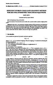
Journal of Applied Mathematics Table 1: Numerical results.

Problem ROSE FROTH BADSCP BADSCB BEALE JENSAM HELIX BARD GAUSS SING WOOD KOWOSB BIGGS OSB2 WATSON ROSEX

SINGX PEN1 PEN2 VARDIM TRIG

BV IE TRID BAND

LIN LIN1

Dim 2 2 2 2 3 2 3 3 3 4 4 4 6 11 20 8 50 100 4 2 4 50 2 50 3 50 100 3 10 200 500 3 200 3 50 100 500 1000 10

MDL 35/349/83 18/88/29 28/275/64 26/446/48 16/87/27 11/31/21 49/347/81 18/38/26 4/9/5 134/501/209 102/613/182 39/178/66 18/279/25 268/1001/445 1455/3587/2274 36/446/90 46/548/101 45/459/99 134/501/209 5/18/12 10/82/26 131/764/254 3/9/7 10/52/36 13/129/27 38/320/70 48/340/90 9/17/11 64/171/97 5/59/7 5/11/7 14/33/18 31/68/39 7/64/12 19/670/26 18/712/27 18/677/26 1/3/3 1/3/3

The step length 𝛼𝑘 in all methods is determined such that the strong Wolfe-Powell conditions (31) and (32) hold with 𝛿 = 0.01 and 𝜎 = 0.1. The test problems are drawn from [14]. The numerical results of our tests are reported in Table 1. The column problem represents the problem name in [14], Dim represents the dimension of the problems. The numerical results are given in the form of 𝐼/𝐹/𝐺, where 𝐼, 𝐹, and 𝐺 denote the numbers of iterations, function evaluations and gradient evaluations, respectively. The stopping condition is ‖𝑔𝑘 ‖ ≤ 10−6 . Since we want to compare the

DL F 9/25/18 36/510/96 F 11/81/22 F 28/164/54 24/145/37 3/7/4 78/396/124 179/865/306 46/383/72 85/564/14 185/888/293 1426/4240/2255 26/421/62 32/469/84 23/445/57 78/396/124 12/182/34 12/89/27 405/1453/683 3/9/7 10/52/36 11/82/25 38/222/68 43/425/76 12/25/16 50/148/81 6/13/8 6/13/8 10/26/17 30/66/37 9/20/13 15/278/23 16/373/26 16/339/27 1/3/3 1/3/3

MHS 38/267/91 15/84/26 42/362/96 28/452/50 14/83/25 11/31/21 47/390/73 18/86/26 4/9/5 111/411/172 207/1352/365 53/259/88 20/286/31 186/701/310 1922/4843/3018 38/362/93 44/412/101 46/414/102 111/411/172 5/18/12 11/133/29 136/1056/256 3/9/7 10/52/36 15/225/27 38/225/71 48/294/90 11/20/13 64/172/99 5/59/7 6/13/8 14/33/18 31/68/39 7/64/12 19/670/26 18/712/27 18/677/26 1/3/3 1/3/3

DY 63/800/106 16/38/26 F F 47/193/74 11/31/21 80/406/126 48/148/77 4/9/5 650/3254/1104 F 462/1760/796 210/644/342 F 548/1480/864 63/764/100 86/707/146 71/856/112 650/3254/1104 5/18/12 32/167/57 121/724/242 3/9/7 10/52/36 162/974/267 206/1662/290 225/3077/286 13/27/18 59/163/93 6/61/8 6/13/8 15/84/21 36/78/42 7/64/12 F F F 1/3/3 1/3/3

performance of the different methods, in the numerical results, we omit the problems if all the four methods perform equally. The notation 𝐹 means that, for this problem, the corresponding method fails.

5. Conclusions In this paper, based on 𝛽𝑘DY and 𝛽𝑘DL , a new formula is proposed to compute the parameter 𝛽𝑘 of the conjugate gradient methods. The main motivations are to improve both

Journal of Applied Mathematics the convergence properties and numerical behavior of the conjugate gradient method. For general conjugate gradient methods, in order to get the global convergence results, the methods are required to possess the following major properties: (1) the generated directions 𝑑𝑘 are descent directions; (2) the parameters 𝛽𝑘 are nonnegative. In addition, to ensure that the methods have robust and efficient numerical behavior, the parameter 𝛽𝑘 needs to approach zero, when the small step 𝑠𝑘 occurs. From the convergence analysis of this paper, we known that the directions 𝑑𝑘 generated by MDL method are descent directions, which is not true for DY or DL methods, and the proposed MDL method is globally convergent for general functions. In the previous section, we compare the numerical performance of the MDL method with the DY, MHS, and DL methods. From the convergence analysis and numerical results, comparing with the DL, DY, and MHS method, we can have the following. (a) MDL method versus DL method: from the computational point of view, for most of the test problems, MDL method performs quite similarly with DL method. There are 15 problems in which MDL method outperforms the DL method and 18 problems in which DL method outperforms the MDL method. But, from the convergent point of view, the MDL method outperforms the DL method. (b) MDL method versus DY method: the convergence properties of MDL method are similar to DY method. By comparing the numerical results of MDL method with DY method, there are 27 test problems in which MDL method outperforms the DY method and only 4 test problems in which DY method outperforms the MDL method. Therefore, we could say that MDL method is much better than the DY method in numerical behavior. (c) MDL method versus MHS method: they possess similar convergence properties; the numerical results show that MDL method performs little better than the MHS method.

Acknowledgments This research was supported by Guangxi High School Foundation Grant no. 2013BYB210 and Guangxi University of Finance and Economics Science Foundation Grant no. 2013A015.

References [1] G. Zoutendijk, “Nonlinear programming, computational methods,” in Integer and Nonlinear Programming, J. Abadie, Ed., pp. 37–86, North-Holland Publishing, Amsterdam, 1970. [2] M. J. D. Powell, “Restart procedures for the conjugate gradient method,” Mathematical Programming, vol. 12, no. 2, pp. 241–254, 1977.

9 [3] M. J. D. Powell, “Nonconvex minimization calculations and the conjugate gradient method,” in Numerical Analysis, vol. 1066 of Lecture Notes in Mathematics, pp. 122–141, Springer, Berlin, Germany, 1984. [4] Y.-H. Dai and L.-Z. Liao, “New conjugacy conditions and related nonlinear conjugate gradient methods,” Applied Mathematics and Optimization, vol. 43, no. 1, pp. 87–101, 2001. [5] J. C. Gilbert and J. Nocedal, “Global convergence properties of conjugate gradient methods for optimization,” SIAM Journal on Optimization, vol. 2, no. 1, pp. 21–42, 1992. [6] G. Li, C. Tang, and Z. Wei, “New conjugacy condition and related new conjugate gradient methods for unconstrained optimization,” Journal of Computational and Applied Mathematics, vol. 202, no. 2, pp. 523–539, 2007. [7] Z. Wei, S. Yao, and L. Liu, “The convergence properties of some new conjugate gradient methods,” Applied Mathematics and Computation, vol. 183, no. 2, pp. 1341–1350, 2006. [8] Y. Shengwei, Z. Wei, and H. Huang, “A note about WYL’s conjugate gradient method and its applications,” Applied Mathematics and Computation, vol. 191, no. 2, pp. 381–388, 2007. [9] H. Huang, S. Yao, and H. Lin, “A new conjugate gradient method based on HS-DY methods,” Journal of Guangxi University of Technology, no. 4, pp. 63–66, 2008. [10] L. Zhang, “An improved Wei-Yao-Liu nonlinear conjugate gradient method for optimization computation,” Applied Mathematics and Computation, vol. 215, no. 6, pp. 2269–2274, 2009. [11] L. Zhang, “Further studies on the Wei-Yao-Liu nonlinear conjugate gradient method,” Applied Mathematics and Computation, vol. 219, no. 14, pp. 7616–7621, 2013. [12] Z. Dai and F. Wen, “Another improved Wei-Yao-Liu nonlinear conjugate gradient method with sufficient descent property,” Applied Mathematics and Computation, vol. 218, no. 14, pp. 7421– 7430, 2012. [13] Y. Dai, J. Han, G. Liu, D. Sun, H. Yin, and Y.-X. Yuan, “Convergence properties of nonlinear conjugate gradient methods,” SIAM Journal on Optimization, vol. 10, no. 2, pp. 345–358, 1999. [14] J. J. Mor´e, B. S. Garbow, and K. E. Hillstrom, “Testing unconstrained optimization software,” ACM Transactions on Mathematical Software, vol. 7, no. 1, pp. 17–41, 1981.

Advances in

Operations Research Hindawi Publishing Corporation http://www.hindawi.com

Volume 2014

Advances in

Decision Sciences Hindawi Publishing Corporation http://www.hindawi.com

Volume 2014

Journal of

Applied Mathematics

Algebra

Hindawi Publishing Corporation http://www.hindawi.com

Hindawi Publishing Corporation http://www.hindawi.com

Volume 2014

Journal of

Probability and Statistics Volume 2014

The Scientific World Journal Hindawi Publishing Corporation http://www.hindawi.com

Hindawi Publishing Corporation http://www.hindawi.com

Volume 2014

International Journal of

Differential Equations Hindawi Publishing Corporation http://www.hindawi.com

Volume 2014

Volume 2014

Submit your manuscripts at http://www.hindawi.com International Journal of

Advances in

Combinatorics Hindawi Publishing Corporation http://www.hindawi.com

Mathematical Physics Hindawi Publishing Corporation http://www.hindawi.com

Volume 2014

Journal of

Complex Analysis Hindawi Publishing Corporation http://www.hindawi.com

Volume 2014

International Journal of Mathematics and Mathematical Sciences

Mathematical Problems in Engineering

Journal of

Mathematics Hindawi Publishing Corporation http://www.hindawi.com

Volume 2014

Hindawi Publishing Corporation http://www.hindawi.com

Volume 2014

Volume 2014

Hindawi Publishing Corporation http://www.hindawi.com

Volume 2014

Discrete Mathematics

Journal of

Volume 2014

Hindawi Publishing Corporation http://www.hindawi.com

Discrete Dynamics in Nature and Society

Journal of

Function Spaces Hindawi Publishing Corporation http://www.hindawi.com

Abstract and Applied Analysis

Volume 2014

Hindawi Publishing Corporation http://www.hindawi.com

Volume 2014

Hindawi Publishing Corporation http://www.hindawi.com

Volume 2014

International Journal of

Journal of

Stochastic Analysis

Optimization

Hindawi Publishing Corporation http://www.hindawi.com

Hindawi Publishing Corporation http://www.hindawi.com

Volume 2014

Volume 2014