Traditional resources in scheduling are simple machines where a capacity is the ... activity B only if there is an arc from the state of A to the state of B in the state ...
A Constraint Model for State Transitions in Disjunctive Resources Roman Barták*, Ondřej Čepek*g *Charles University, Faculty of Mathematics and Physics Malostranské nám. 2/25, 118 00 Praha 1, Czech Republic {roman.bartak,ondrej.cepek}@mff.cuni.cz gInstitute of Finance and Administration Estonská 500, 101 00 Praha 10, Czech Republic
Abstract Traditional resources in scheduling are simple machines where a capacity is the main restriction. However, in practice there frequently appear resources with more complex behaviour that can be described using state transition diagrams. This paper presents new filtering rules for constraints modelling the state transition diagrams. These rules are based on the idea of extending traditional precedence graphs by direct precedence relations. The proposed model also assumes optional activities and it can be used as an open model accepting new activities during the solving process.
Introduction Temporal networks play an important role in planning but they are not used as frequently in scheduling where resource restrictions traditionally play a stronger role. This is reflected in scheduling global constraints, where techniques like edge-finding or not-first/not-last combine restrictions on time windows with a limited capacity of the resource (Baptiste, Le Pape, Nuijten 2001). Recently, a new category of propagation techniques combining information about relative position of activities with capacity of resources appeared (Cesta and Stella 1997). Also techniques combining information about precedence relations and time windows have been proposed (Laborie 2003). We believe that integration of temporal networks with reasoning on resources (Laborie 2003b; Moffit, Peintner, and Pollack 2005) will play even more important role as planning and scheduling technologies are becoming closer. In this paper we propose an extension of precedence graphs by direct precedence relations (A can directly precede B if no activity must be allocated between A and B). This extension is motivated by modelling complex behaviour of resources that is described as a state transition diagram. Such a diagram is in fact a generalisation of setup times that play an important role in current real-life scheduling problems. As factories are transforming from mass production to more customised production, multipurpose and hence more complicated machines are used and better handling of setups is becoming important. Space applications are another example where a more complex
behaviour of resources is typical. Also over-subscribed problems are more frequent nowadays so the scheduling systems are not just allocating activities to time and resources but also decide about rejection of activities that cannot be scheduled feasibly together with other activities. Such problems can be modelled by optional activities, where the scheduling system decides about their presence (validity) in the final schedule. Note also, that optional activities are useful for modelling alternative resources (an optional activity is used for each alternative resource) as well as alternative processes to accomplish a job (each process may consist of one of several different sets of activities). Scheduling systems should also be able to add activities to satisfy the transition scheme, for example to insert a setup activity if necessary. To summarise the contributions of this paper, we propose two extensions of ordinary precedence graphs: adding direct precedence relations and using optional activities. For such a graph which we call a double precedence graph we design incremental filtering rules that keep a transitive closure of the graph and deduce new precedences and (in)validity of activities. Moreover, in contrast to traditional global constraints used in scheduling the proposed model is open, that is, it allows adding new activities to the precedence graph during the solution process.
Motivation In this paper we address the problem of modelling a disjunctive resource where activities must be allocated in such a way that they do not overlap in time. In other words, the disjunctive resource can process at most one activity at any time (such resources are also called unary). We assume that there are precedence constraints between the activities. The precedence constraint A « B specifies that activity A must finish before activity B starts in the schedule. The relation between two activities A and B allocated to a disjunctive resource can now be described using a constraint A « B or B « A. Each activity is annotated by a resource state requested for processing the activity and there is a state transition diagram describing transitions between the states. State transition diagram is a directed
graph where nodes describe the states and arcs describe allowed transitions between the states (Figure 1). The state transition diagram restricts sequencing of activities in the following way: activity A can be scheduled directly before activity B only if there is an arc from the state of A to the state of B in the state transition diagram. To model oversubscribed problems and alternative resources/processes, we assume optional activities. An optional activity has one of the following three statuses. If the activity is not yet known to be or not to be included then it is called undecided. If the activity is allocated to the resource then it is called valid. If the activity is known not to be allocated to the resource then it is called invalid. Regular activities correspond to valid activities. The scheduling task is to decide about (in)validity of the undecided activities and to find a sequence of valid activities satisfying the precedence constraints and restrictions imposed by the state transition diagram. target location
download picture position antenna
take picture
store picture
Figure 1. Example of a state transition diagram.
In this paper we focus on modelling restrictions imposed by the precedence relations and by the state transition diagram. In other words, we are interested in sequencing of activities rather than in their absolute positioning in time. Nevertheless, at the end of the paper we will show how the proposed approach can be combined with reasoning on time windows as presented in (Barták 2006).
Related Works Disjunctive temporal networks (Stergiou and Koubarakis 1998) can model disjunctive resources. However, DTNs use more general disjunctions than necessary and hence they achieve weaker pruning. Moreover, a qualitative approach to time seems more appropriate to describe the problem of activity sequencing. Though we assume durative activities, Interval Algebra is superfluous because disjunctive resources discard most of the interval relations (like starts, during, overlaps etc.). From Point Algebra we need only ‘before’ and ‘after’ relations and there is no support for direct precedences there. The work by Laborie (2003b) studies a combination of resource and temporal reasoning but no algorithm is presented (and a different type of resources is assumed). Probably the closest approach to our problem is presented in the paper (Focacci, Laborie, and Nuijten 2000) where alternative resources correspond to paths in the global precedence graph. However, this approach is proposed merely for cost-based filtering (optimization of makespan or setup times) and it
assumes all the activities to be present in the global precedence graph. The paper (Beck and Fox 1999) presents an idea of a precedence graph with optional activities. The authors use a so called PEX value to describe a probability of the existence of the activity and their approach is based on updating this value. Instead of that we use a Boolean variable to describe the presence of an activity and we focus more on precedence and direct precedence relations. To summarise the above discussion, none of the existing approaches to temporal and resource reasoning covers fully state transition diagrams simultaneously with optional activities.
Double Precedence Graphs The precedence relations among activities define a precedence graph that is an acyclic directed graph where nodes correspond to activities and there is an arc from A to B if A « B. If access to all predecessors and successors of a given activity is frequently requested, like in (Cesta and Stella 1997; Laborie 2003), then it is more efficient to keep a transitive closure of the graph where this information is available in time O(1) rather than to look for predecessors/successors on demand. We propose the following definition of transitive closure of the precedence graph with optional activities. Definition 1: We say that a precedence graph G with optional activities is transitively closed if for any two arcs A to B and B to C such that B is a valid activity and A and C are either valid or undecided activities there is also an arc A to C in G. It is easy to prove that if there is a path from A to B such that A and B are either valid or undecided and all inner nodes in the path are valid then there is also an arc from A to B in a transitively closed graph (by induction on the path length). Hence, if no optional activity is used (all activities are valid) then Definition 1 corresponds to a standard definition of the transitive closure. To model restrictions imposed by the state transition diagram we propose to extend the precedence graph by direct precedence relations between the activities. Definition 2: We say that A can directly precede B if both A and B are either valid or undecided activities, B is not before A (¬ B « A), the transition from A to B is allowed by the state transition diagram, and there is no valid activity C such that A « C and C « B (the relation « is from the transitive closure of the precedence graph with optional activities). The relation of direct precedence introduces a new type of arc, say «d, in the precedence graph and hence we are speaking about the double precedence graph. There is one significant difference between the arcs of type « and the arcs of type «d. While the arcs « are added into the graph as problem solving proceeds, the arcs «d are typically removed from the graph (note that «d means “can be directly before”, while « means “must be before”). When
all valid activities are linearly ordered, there is exactly one arc of type «d going into each valid activity (with the exception of the very first activity in the schedule) and one arc of type «d going from each valid activity (with the exception of the very last activity in the schedule).
Constraint Model We propose to realise a reasoning on precedence relations using constraint satisfaction technology. This allows integration of our model with other constraint reasoning techniques (Barták 2006). This integration requires the model to provide full information about precedence relations to all other constraints. We index each activity by a unique number from the set 1,..,n, where n is the number of activities. For each activity we use a 0/1 variable Valid indicating whether the activity is valid (1) or invalid (0). If the activity is undecided – not yet known to be valid or invalid – then the domain of Valid is {0,1}. The precedence graph is encoded in two sets attached to each activity. CanBeBefore(A) is a set of indices of activities that can be before activity A. CanBeAfter(A) is a set of indices of activities that can be after activity A. For simplicity reasons we will write A instead of the index of A. To simplify description of the propagation rules we define for every activity A the following derived sets: MustBeAfter(A) = CanBeAfter(A) \ CanBeBefore(A) MustBeBefore(A) = CanBeBefore(A) \ CanBeAfter(A) Unknown(A) = CanBeBefore(A) ∩ CanBeAfter(A). MustBeAfter(A) and MustBeBefore(A) are sets of those activities that must be after and before the given activity A respectively. Unknown(A) is a set of activities that are not yet known to be before or after activity A (Figure 2). To model direct precedence relations and hence a double precedence graph, we add two sets to each activity A: CanBeRightBefore(A) and CanBeRightAfter(A) with indices of activities that can be directly before and directly after a given activity. Naturally, the following relation holds CanBeRightBefore(A) ⊆ CanBeBefore(A) at any time and similarly CanBeRightAfter(A) ⊆ CanBeAfter(A). CanBeBefore(A) Unknown(A) MustBeAfter(A)
MustBeBefore(A)
A CanBeAfter(A)
Figure 2. Representation of the precedence graph.
Note on representation. The main reason for using sets to model the precedence graph is their possible representation as domains of variables in constraint satisfaction packages. Recall that domains of variables can only shrink as problem solving proceeds. The sets in our model are also
shrinking as new arcs « are added to the precedence graph. Hence a special data structure is not necessary to describe the precedence graph in constraint satisfaction packages. Moreover, these packages usually provide tools to manipulate the domains, for example membership and deletion operations. In the subsequent complexity analysis, we will assume that these operations require time O(1), which can be realised for example by using a bitmap representation of the sets. Note finally, that empty domain implies inconsistency that may be a problem for the very first and very last activity which has no predecessors and successors respectively. To solve the problem we can simply leave activity A in both sets CanBeAfter(A) and CanBeBefore(A) and similarly for direct precedences. Then no domain of CanBeBefore and CanBeAfter will ever be empty but we can detect inconsistency via the empty domain of Valid variables.
Propagation Rules for Simple Precedences The goal of propagation rules is to remove inconsistent elements (activities) from the above described sets – this is called domain filtering in constraint satisfaction. In the first stage, we will focus on making a transitive closure of the precedence graph according to Definition 1. Note that the transitive closure of the precedence graph also simplifies detection of inconsistency of the graph. The precedence graph is inconsistent if there is a cycle of valid activities. In a transitively closed graph, each such cycle can be detected by finding two valid activities such that A « B and B « A. Our propagation rules prevent cycles by making invalid the last undecided activity in each cycle. This propagation is realised by using an exclusion constraint. As soon as there is a cycle A « B and B « A detected, the following exclusion constraint can be posted: Valid(A) = 0 ∨ Valid(B) = 0. This constraint ensures that each cycle is broken by making at least one activity in the cycle invalid. Instead of posting the constraint directly to the constraint solver, we propose keeping the set Ex of exclusions. The above exclusion constraint is modelled as a set {A,B} ∈ Ex. Now, the propagation of exclusions is realised explicitly – if activity A becomes valid then all activities C such that {A,C} ∈ Ex are made invalid. We initiate the precedence graph in the following way. First, the variables Valid(A), CanBeBefore(A), CanBeRightBefore(A), CanBeAfter(A), and CanBeRightAfter(A) with their domains are created for every activity A. Then the known precedence relations in the form A « B are added by removing B from the sets CanBeBefore(A) and CanBeRightBefore(A), and removing A from the sets CanBeAfter(B) and CanBeRightAfter(B). Note, that because all activities are still undecided at this stage, domain change is not propagated to other variables. Finally, the Valid(A) variable for every valid activity A is set to 1 (and similarly Valid variables of invalid activities are set to 0). When an activity becomes invalid, it is removed from the graph
which is realised by removing it from all the sets. When an activity becomes valid then all activities that form exclusion with it are made invalid. Additionally, the noninvalid predecessors of the activity are connected to the non-invalid successors of the activity to keep the transitive closure (by non-invalid activity we mean undecided or valid activity). Possible cycles are detected at this stage and some direct precedences are removed. This reasoning is realised by the following propagation rule /1/ which is called whenever the Valid variable is instantiated. “Valid(A) is instantiated” is its trigger. The part after is a propagator describing pruning of domains. “exit” means that the constraint represented by the propagation rule is entailed so the propagator is not further invoked (its invocation does not cause further domain pruning). We will use the same notation in all rules. The propagation rule /1/ realises the above described exclusion constraints as well as adding new arcs according to Definition 1. Valid(A) is instantiated /1/ if Valid(A) = 0 then Ex := Ex \ {{A,X} | X is an activity} for each B do // disconnect A from B CanBeBefore(B) ← CanBeBefore(B) \ {A} CanBeAfter(B) ← CanBeAfter(B) \ {A} CanBeRightBefore(B) ← CanBeRightBefore(B) \ {A} CanBeRightAfter(B) ← CanBeRightAfter(B) \ {A} else // Valid(A)=1 for each C s.t. {A,C}∈Ex do Valid(C) ← 0 for each B∈MustBeBefore(A) s.t. Valid(B)≠0 do for each C∈MustBeAfter(A) s.t. Valid(C)≠0 do CanBeRightAfter(B) ← CanBeRightAfter(B) \ {C} CanBeRightBefore(C) ← CanBeRightBefore(C) \ {B} if C∉MustBeAfter(B) then CanBeAfter(C) ← CanBeAfter(C) \ {B} //add arc from B to C CanBeBefore(B) ← CanBeBefore(B) \ {C} CanBeRightAfter(C) ← CanBeRightAfter(C) \ {B} CanBeRightBefore(B) ← CanBeRightBefore(B) \ {C} if C∉CanBeAfter(B) then // break the cycle if Valid(B)=1 then Valid(C) ← 0 // Valid(C)=1 leads to fail else if Valid(C)=1 then Valid(B) ← 0 else Ex ← Ex ∪ {{B,C}} exit
Note that rule /1/ maintains symmetry of sets modelling the double precedence graph for all valid and undecided activities because the domains are pruned symmetrically in pairs. It is possible to show, that if the entire precedence graph is known in advance (no arcs are added during the solving procedure), then rule /1/ is sufficient for keeping the transitive closure according to Definition 1. In particular, if there is a path between non-invalid nodes A and B such that all inner nodes of the path are valid then there is an arc between A and B. The worst-case time complexity of the propagation rule /1/ (instantiation of the Valid variable) including all possible recursive calls is O(n2), where n is the number of activities. The formal proofs can be found in (Barták & Čepek, 2006). In some situations arcs may be added to the double precedence graph during the solving procedure, either by the user, by the scheduler/planner, or by other filtering
algorithms like the one proposed in (Barták 2006). The following rule /2/ updates the double precedence graph to keep transitive closure when an arc is added to the double precedence graph. If a new arc A«B is added then we first check whether the arc is not already present in the graph. If it is a new arc then the corresponding sets are updated and a possible cycle is detected (we use the same reasoning as in rule /1/). Finally, if any end point of the arcs is valid, then necessary arcs are added to update the transitive closure according to Definition 1. In such a case, some direct precedence relations are removed according to Definition 2 (like in rule /1/). Note that the propagators for new arcs are evoked after the propagator of the current rule finishes. A«B is added /2/ if A∈MustBeBefore(B) then exit // the arc is already present CanBeAfter(B) ← CanBeAfter(B) \ {A} CanBeBefore(A) ← CanBeBefore(A) \ {B} CanBeRightAfter(B) ← CanBeRightAfter(B) \ {A} CanBeRightBefore(A) ← CanBeRightBefore(A) \ {B} if A∉CanBeBefore(B) then // break the cycle if Valid(A)=1 then Valid(B) ← 0 // Valid(B)=1 leads to fail else if Valid(B)=1 then Valid(A) ← 0 // Valid(A)=1 leads to fail else Ex ← Ex ∪ {{A,B}} else // transitive closure if Valid(A)=1 then for each C∈MustBeBefore(A) s.t. Valid(C)≠0 do CanBeRightAfter(C) ← CanBeRightAfter(C) \ {B} CanBeRightBefore(B) ← CanBeRightBefore(B) \ {C} if C∉MustBeBefore(B) then add C«B if Valid(B)=1 then for each C∈MustBeAfter(B) s.t. Valid(C)≠0 do CanBeRightAfter(A) ← CanBeRightAfter(A) \ {C} CanBeRightBefore(C) ← CanBeRightBefore(C) \ {A} if C∉MustBeAfter(A) then add A«C exit
Again, it is possible to show that if the precedence graph G is transitively closed (in the sense specified by Definition 1) and arc A « B is added to G then rule /2/ updates the precedence graph G to be transitively closed again. Note also, that propagation rules /1/ and /2/ achieve global consistency concerning the precedence constraint. It means that if A and B are two non-invalid activities and A∈CanBeBefore(B) then there exists a feasible schedule where both A and B are valid and A is before B. This is a direct consequence of keeping a transitive closure of the precedence graph. Moreover, the information about direct precedence relations is kept consistent. Namely, if A and B are two non-invalid activities and B « A or there is a valid activity C between A and B (that is, A « C and C « B) then A∉CanBeRightBefore(B) and B∉CanBeRightAfter(A). The worst-case time complexity of the propagation rule /2/ (adding a new arc) including all recursive calls to rules /1/ and /2/ is O(n3), where n is the number of activities. The formal proofs can be found in (Barták & Čepek, 2006).
A Propagation Rule for Direct Precedences So far we more or less ignored the restrictions imposed by the state transition diagram. The reason is that these restrictions can be easily encoded by removing explicitly direct precedence relations from the double precedence graph. In particular, if transition from A to B is forbidden by the state transition diagram then arc A «d B is removed from the double precedence graph. In a linearly ordered set of activities it implies that there must be some valid activity C between A and B or B must be after A. Actually a stronger requirement can be imposed: if A is before B (and A cannot be directly before B) then there must be some valid activity directly before B that is also after A and some valid activity directly after A that is before B. This observation can be transformed into the following implications: CanBeRightAfter(A) ∩ CanBeBefore(B) = ∅ ⇒ B « A CanBeAfter(A) ∩ CanBeRightBefore(B) = ∅ ⇒ B « A. The above reasoning can be used to deduce a new precedence constraint B « A and, vice versa, if A « B then we can actively look for activities between A and B, especially, if there is only one candidate for such activity. This reasoning is realised using two propagation rules. First, the direct precedence is removed using rule /3/ and rule /4/ is activated. Rule /4/ is then called whenever there are some changes related to activities A or B. This rule tries to deduce that B must be before A or if A « B then the rule looks for some activity C between A and B. Notice that opposite to rules /1/-/3/, rule /4/ can be invoked repeatedly until it deduces B « A or finds activity C such that A « C and C « B. Moreover, rule /4/ is active only when rule /3/ activates it for particular activities A and B. A«dB is deleted /3/ CanBeRightAfter(A) ← CanBeRightAfter(A) \ {B} CanBeRightBefore(B) ← CanBeRightBefore(B) \ {A} activate rule /4/ for A and B exit CanBeRightAfter(A) or CanBeAfter(A) or CanBeBefore(A) or CanBeRightBefore(B) or CanBeBefore(B) or CanBeAfter(B) is changed, or Valid(A) or Valid(B) is instantiated /4/ if Valid(A)=0 or Valid(B)=0 or A∈MustBeAfter(B) then exit if CanBeRightAfter(A)∩CanBeBefore(B)=∅ or CanBeAfter(A)∩CanBeRightBefore(B)=∅ then add B«A exit if A∈MustBeBefore(B) & Valid(A)=1 & Valid(B)=1 then if {C}= CanBeRightAfter(A)∩CanBeBefore(B) or {C}= CanBeAfter(A)∩CanBeRightBefore(B) then // C is the only possible direct successor of A or // C is the only possible direct predecessor of B add A«C add C«B Valid(C) = 1 exit
If there are no explicit direct precedence relations like those imposed by the state transition diagram, then we already showed that propagation rules /1/-/2/ achieve
global consistency. Unfortunately, in general, global consistency is not achieved by rules /3/-/4/, that is, for explicitly removed direct precedence relations. It means that even if the problem is locally consistent (the propagation rules do not make any domain/set empty) it does not imply that there exists a solution. In such a case, search procedure can be involved. Nevertheless, we can show that the constraint realised by rules /3/-/4/ is complete. Namely, if all activities are either valid or invalid and the set of valid activities is totally ordered then this order satisfies the restrictions imposed by the state transition diagram. The worst-case time complexity of the propagation rule /4/ including all recursive calls to rules /1/ and /2/ is O(n3), where n is a number of activities. Again, the formal proofs can be found in (Barták & Čepek, 2006).
Possible Extensions So far, we focused on handling precedence and direct precedence relations only. In this section, we will show how information about precedence relations can be combined with reasoning on time windows and how the precedence graph can be open to accept new activities during problem solving.
Combining Time Windows with Precedences As mentioned in the motivation, we are addressing the problem of scheduling activities on a disjunctive resource, that is, a resource that can process at most one activity at any time. Many filtering algorithms have been proposed for such type of resources, for example edge-finding or not-first/not-last techniques (Baptiste, Le Pape, Nuijten 2001). A common feature of these algorithms is that they are working primarily with time windows, namely, they are increasing the earliest start time (est) and decreasing the latest completion time of activities (lct). As an intermediate step, these algorithms can also deduce some precedence relations, for example, the edge-finding technique deduces that some activity must be processed before or after a set of other activities. Other precedences can be deduced simply by looking at time windows of activities, these precedences are called detectable. Assume that est(X) is the earliest start time of activity X, lct(X) is the latest completion time of activity X, and p(X) is a duration of activity X. If est(A) + p(A) + p(B) > lct(B) then activity A cannot be processed before activity B and hence we can deduce B « A (Figure 3). So, information about time windows can be used to deduce precedence relations that can be included in the double precedence graph. Consequently, using time windows can strengthen reasoning on precedence relations. 0
B (pB=11) 14
25
A (pA=5)
Figure 3. Detectable precedence B « A
35
On the other hand, information about precedence relations can be used to shrink time windows as shown in (Laborie 2003) and (Barták 2006). Assume that we have a set of valid activities Ω that must be processed before some activity C. Let us define the earliest start time of Ω as the minimal earliest start of activities in Ω and duration of Ω as the sum of durations of activities in Ω. Formally: est(Ω)= min{est(A) | A∈Ω}, p(Ω)= ∑{p(A) | A∈Ω}. Clearly, the earliest completion time when all activities in Ω are finished is est(Ω) + p(Ω). Because C is processed after all activities in Ω, C cannot start before the earliest completion time of Ω (Figure 4). This deduction can be applied to any subset of valid activities that must be processed before C so we can obtain a better estimate of the earliest start time of C. Similarly, we can use the valid activities after C to deduce a better estimate of its latest completion time. Formally: est(C) ← max{est(Ω)+p(Ω) | Ω⊆{X | X«C ∧ Valid(X)=1}} lct(C) ← min{lct(Ω)-p(Ω) | Ω⊆{X | C«X ∧ Valid(X)=1}} This way, the information about precedence relations can be used to shrink time windows. Note also, that this reasoning can deduce other changes than the algorithms based purely on time windows so both approaches, namely reasoning on time windows and reasoning on precedence relations, can be combined to prune more the search space. Ω 0
25
A (pA=11) 1
A«C
27
B (pB=10) 14
B«C
C (pC=5)
35
This computation can be realised in time O(n.log n) using the following algorithm. The new bound for est(C) is computed in the variable end. dur ← 0 end ← inf // infimum = minus infinity for each Y∈{X | X « C ∧ Valid(X) = 1} in the non-increasing order of est(Y) do dur ← dur + p(Y) end ← max(end, est(Y) + dur)
We need time O(n.log n), where n is the number of activities, to sort the activities and time O(n) for the loop. The bound for lct(C) can be computed in a symmetrical way in time O(n.log n). The paper (Barták 2006) shows how this reasoning can be realised in the form of filtering rules similar to rules presented in this paper.
Sequence-dependent Setup Times The original motivation for introducing direct precedence relations into precedence graphs was modeling sequence dependent setup times. Setup time is a time that is necessary to be inserted between two consecutive activities to setup the machine. If this setup time depends on both activities then it is called a sequence-dependent setup time. Typically, setup time is assumed to be an empty gap between two consecutive activities. Our idea is to include the setup time in the duration of the second activity. Basically, it means that duration of each activity will consists of its real duration plus a setup time (Figure 5). Clearly because of time windows we still need to keep the original start time of the activity but we add the extended start time to model the start time including the setup. The extended start time can then participate in non-overlapping constraints for disjunctive resources like edge-finding without modifying these constraints.
21 = 0+11+10
Figure 4. From precedences to pruning time windows
It may seem that the above described reasoning requires exploring all subsets Ω which would lead to an exponential time complexity. Nevertheless, this is not the case and, as shown for example in (Vilím et al. 2005), the bounds for time windows can be computed in time O(n.log n), where n is the number of activities. Let Ω’ be the subset of the set {X | X « C ∧ Valid(X) = 1} with the maximal earliest completion time est(Ω’) + p(Ω’). In other words, set Ω’ defines the new bound for est(C). Then Ω’must contain all activities {X | X « C ∧ Valid(X) = 1 ∧ est(Ω’) ≤ est(X)}, because otherwise adding such X to Ω’ will increase p(Ω’) and hence also est(Ω’) + p(Ω’). Consequently, when computing the bound for est(C), it is enough to explore sets Ω〈X,C〉 = {Y | Y « C ∧ Valid(Y) = 1 ∧ est(X) ≤ est(Y)} for each valid X that must be before C. In particular, the new bound est(C) is computed using the formula: max{ est(Ω〈X,C〉) + p(Ω〈X,C〉) | X « C ∧ Valid(X) = 1 }.
extended start time SETUP
end time
start time
ACTIVITY
Figure 5. From precedences to pruning time windows
The difference between the start time and the extended start time equals exactly to the setup time for a given activity (for the first activity, we can use a startup time). To find out the setup time we can use information about direct predecessors of the activity. Because we are working in the context of constraint satisfaction, we can use a binary constraint between the variable describing a direct predecessor (CanBeRightBefore) and the variable describing the setup time. The relation behind this constraint is extensionally defined – it is a list of setup times for the activity where index of each element corresponds to identification of the possible predecessor. Note finally, that these ideas can be included in filtering of times windows; we just need to assume variable duration.
Open Graphs The double precedence graphs studied in previous sections assume that the number of activities or at least its upper estimate is known. We use optional activities to deactivate activities that will not be part of the solution. This technique is appropriate in scheduling applications where most activities are known and optional activities are used to model alternatives to be decided during scheduling. However, in planning this technique is less convenient because the number of activities is unknown. It is still possible to use optional activities but in this case, the total number of activities will be probably too large which will decrease overall efficiency. Our constraint model can be used directly to include new activities that will appear during problem solving. Recall, that we model the double precedence graph using difference sets, in particular the set CanBeBefore(A)\CanBeAfer(A) describes the activities that must be before A. We assumed that these sets are subsets of {1,…, n}, where n is the number of activities. To model problems where the number of activities is unknown in advance, we can use an infinite set {1,…,sup}, where sup is a computer representation of “plus infinity”. The activities, that are already known, are represented using the variable Valid and sets CanBeBefore and CanBeAfter. The other activities are represented just by their indices in these sets. Hence, these activities behave like optional undecided activities with no precedence relations to activities already in the graph. Therefore, there is no propagation related to these activities so sets representing these activities are not changing and hence it is not necessary to keep them in memory (only indices of invalid activities may be deleted from these sets, but it does not play any role). As soon as a new activity is included in the precedence graph then an index is assigned to the activity and its set representation is created. At this time all invalid activities should be removed from the sets of the new activity. We only need to keep the number of activities already included in the precedence graph to know which index can be used. Note finally, that we can still use optional activities to model alternatives to be decided later. In addition to adding activities from outside, it is possible to use the double precedence graph to deduce that a new activity must be added to the graph. In particular, if A « B but A cannot be directly before B and no existing activity is between A and B then we can deduce that a new activity C must be added together with the precedence relations A « C and C « B. This might be useful especially to resolve flaws in plan-space planning.
Experimental Results We are currently working on implementation of the proposed filtering algorithms. We have already implemented the model of the precedence graph with optional activities in SICStus Prolog 3.12.3 using the standard interface for the definition of global constraints.
In this section, we present some preliminary experimental results comparing our approach with the constraints model from (Fages 2001) using min-cutset problems. A mincutset problem consists of precedence relations and the task is to find the largest set of vertices such that the subgraph induced by these vertices does not contain any cycle (or symmetrically to find the smallest set of vertices such that all cycles are broken if these vertices are removed from the graph). This problem is known to be NP-hard (Garey and Johnson 1979). We use the data set from (Pardalos, Qian, and Resende 1999) to compare our approach based on the precedence graph with the CLP model from (Fages 2001) based on absolute positioning in the sequence of activities (Original). The model uses n integer variables p1,…, pn giving the absolute position of activities in the schedule (n is the number of activities). The initial domain of these variables is 1,…,n. There are also n Boolean (0/1) variables a1,…, an describing whether the activity is valid (1) or invalid (0). The precedence constraint between activities i and j is then described using the formula: (ai ∧ aj) => (pi < pj) or equivalently (ai * aj * pi < pj). All the problems in the data set consist of 50 activities while the number of precedence constraints varies. Table 1 shows the specification of problems used in our experiment and the best solutions obtained. Note that the solutions obtained by our approach (Precedence) are optimal. The experiments run under Windows XP Professional on 1.1 GHz Pentium-M processor with 1280 MB RAM. Bench
Activities
Precedences
Original
Precedence
P50-100
50
100
47
47
P50-150
50
150
41
41
P50-200
50
200
35
37
P50-250
50
250
31
33
P50-300
50
300
28
31
P50-500
50
500
21
22
P50-600
50
600
17
19
P50-700
50
700
16
17
P50-800
50
800
16
16
P50-900
50
900
14
14
Table 1. Min-cutset problems.
Figure 6 shows the comparison of runtimes and Figure 7 shows the number of backtracks to find and prove optimal solutions. Our approach requires more than an order of magnitude less backtracks and less runtime to find and prove the optimal solution. In fact, with the exception of problems with 100 and 150 precedence constraints, the original CLP model was not able to find the optimal solution (or to prove optimality) within the time limit of 50 minutes. The experiments show that reasoning on relative position of activities provides better efficiency than a simple model based on absolute positioning of activities.
10000000
References
Backtracks
1000000 100000 10000 1000 Original
100
Precedence
10 0
200
400
600
800
1000
Number of precedences
Figure 6. The number of backtracks on min-cutset problems 10000000
Runtime (ms)
1000000 100000 10000 Original
1000
Precedence
100 0
200
400
600
800
1000
Number of precedences
Figure 7. The runtime on min-cutset problems
Conclusions In the paper, we introduced a new constraint model describing precedence graphs with optional activities and direct precedence relations. For this model we proposed propagation rules that keep a transitive closure of the graph and remove inconsistencies caused by forbidden direct precedence relations. The forbidden direct precedences are defined by the state transition diagram but they can also come from other sources, for example to remove threats in plan-space planning. We also showed several extensions of this model, namely integration with reasoning on time windows and opening the precedence graph for new activities. Though the paper presents a technology rather than a particular space application, we believe that it might be appropriate for space applications like scheduling earth observations especially because the proposed technology is designed for resources with more complex behaviour.
Acknowledgements The research is supported by the Czech Science Foundation under the contract no. 201/04/1102.
Baptiste, P.; Le Pape, C.; and Nuijten, W. 2001. Constraint-Based Scheduling: Applying Constraint Programming to Scheduling Problems. Kluwer Academic Publisher. Barták, R. 2006. Incremental Propagation of Time Windows on Disjunctive Resources. In Proceedings of the Nineteenth International Florida Artificial Intelligence Research Society Conference (FLAIRS 2006), pp. 25-30. Barták, R. and Čepek, O. 2006. A Constraint Model for State Transitions in Disjunctive Resources. Institute for Theoretical Computer Science. ITI Report 2006-306. 2006. Beck, J.Ch. and Fox, M.S. 1999. Scheduling Alternative Activities. Proceedings of AAAI-99, USA, pp. 680-687. Cesta, A. and Stella, C. 1997. A Time and Resource Problem for Planning Architectures, Recent Advances in AI Planning, LNAI 1348, Springer Verlag, pp. 117-129. Fages, F. 2001. CLP versus LS on log-based reconciliation problems for nomadic applications. In Proceedings of ERCIM/CompulogNet Workshop on Constraints, Praha. Focacci, F.; Laborie, P.; and Nuijten, W. 2000. Solving Scheduling Problems with Setup Times and Alternative Resources. In Proceedings of AIPS 2000. Garey, M. R. and Johnson, D. S. 1979 Computers and Intractability: A Guide to the Theory of NP-Completeness. W. H. Freeman and Company, San Francisco. Laborie, P. 2003. Algorithms for propagating resource constraints in AI planning and scheduling: Existing approaches and new results. Artificial Intelligence 143: 151-188. Laborie, P. 2003b. Resource temporal networks: Definition and complexity. In Proceedings of the 18th International Joint Conference on Artificial Intelligence, pp. 948-953. Moffitt, M. D.; Peintner, B.; and Pollack, M. E. 2005. Augmenting Disjunctive Temporal Problems with FiniteDomain Constraints. In Proceedings of the 20th National Conference on Artificial Intelligence (AAAI-2005), pp. 1187-1192. AAAI Press. Stergiou, K., and Koubarakis, M. 1998. Backtracking algorithms for disjunctions of temporal constraints. In Proceedings of the 15th National Conference on Artificial Intelligence (AAAI-98), pp. 248-253. AAAI Press. Pardalos, P.M.; Qian, T.; Resende, M.G. 1999. A greedy randomized adaptive search procedure for the feedback vertex set problem. Journal of Combinatorial Optimization, 2:399-412. Vilím, P.; Barták R.; and Čepek O. 2005. Extension of O(n.log n) Filtering Algorithms for the Unary Resource Constraint to Optional Activities, Constraints, Volume 10, Number 4, 403-425.