A constructive law of large numbers with application to countable Markov chains Peter G´acs Boston University
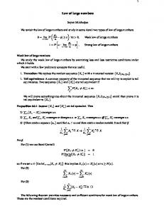
[email protected] December 31, 2010 Abstract Let X1 , X2 , . . . be a sequence of identically distributed, pairwise independent random variables with distribution P. Let the expected value be µ < ∞. Let S n = ∑ni=1 Xi . It is well-known that S n /n converges to µ almost surely. We show that this convergence is effective in (P, µ). In particular, if P, µ are computable then the convergence is effective. On the other hand, if the convergence is effective in P then µ is computable from P. The effectiveness of convergence is detached in the sense that nothing can be inferred about the speed of convergence in the law of large numbers from the speed of convergence in computing P and µ. This theorem can be used to show an effective renewal theorem, which then can be used to prove an effective ergodic theorem for countable Markov chains. The last result is a special case of effective ergodic theorems proven by Avigad-Gerhardy-Towsner and Galatolo-Hoyrup-Rojas, but we hope that the direct constructivization of the probability-theory proofs is still useful.
1
Introduction
The paper [7] gives an example of a countable Markov chain with a computable distribution, for which the convergence of relative frequencies to their limit, guaranteed by the ergodic theorem, is provably non-effective. The author has been intrigued by this example, since the Markov chain given there is not ergodic. The present note is devoted to showing that for ergodic Markov chains,
2 the convergence is constructive. This is a special case of effective ergodic theorems proven in [1] and simplified in [3], but we hope that the direct constructivization of the probability-theory proofs is still useful. Along the way, we explore constructive content of the law of large numbers and some related theorems of probability theory. In the most frequently used laws of large numbers, in which some higher moments are assumed to exist, speed of convergence is simple, and is an important part of the statement and the proof. But in case of identically distributed, (pairwise) independent variables, the law of large numbers follows already from the existence of the expected value. This is the version we need for countable Markov chains, and in this case, the question of speed of convergence is more subtle. Let X1 , X2 , . . . be a sequence of identically distributed, pairwise independent random variables with distribution P. Let the expected value be µ < ∞. Let S n = ∑ni=1 Xi . It is well-known that S n /n converges to µ almost surely. We show that this convergence is effective in (P, µ). In particular, if P, µ are computable then the convergence is effective. On the other hand, if the convergence is effective in P then µ is computable from P. To a probabilist, the theorem should sound unnatural, and with good reason. Fixing the computability of P, it said that the existence of a computable speed of convergence in the law of large numbers depends on whether µ is computable. This suggests that a faster way of computing µ will result in faster convergence in the law of large numbers. But this is not so. Even with P(x) concentrated on positive integers, taking binary rational values computable in linear time from x, and even with µ = 1, the convergence in the law of large numbers can be arbitrarily slow.
2
Computable random variables
We assume familiarity with computable probability spaces, see [5]. Notation 2.1. We will denote the expected value with respect to distribution P by E P , but if (as in most cases) the distribution P is obvious from the context then we will omit the subscript. The same convention is used for the variance Var P . y Definition 2.2. A random variable is computable if its distribution over R is a computable measure. A sequence X1 , X2 , . . . of random variables is computable
3 if all finite joint distributions are uniformly computable.
y
The following observation seems useful. Proposition 2.1. A random variable X is computable if and only if both the distribution function F(x) = P[ X < x ] of X and the distribution function G(x) of −X are lower semicomputable. Proof. The “only if” part is is immediate. For the “if” part, by a theorem of Hoyrup-Rojas in [5], the random variable X is computable if and only if all probabilities of the form P[ a < X < b ] for rational a < b are lower semicomputable. Now P[ a < X < b ] = P[ X < b ] − P[ X 6 a ] = F(x) + G(−a) − 1.
The expected value of a probability distribution is necessarily lower semicomputable as a function of the distribution P. The following proposition is frequently used. Proposition 2.2. Let X be a nonnegative random variable with distribution funcR∞ tion F(x) = P[ X < x ], then E P X = 0 (1 − F(x))dx. In particular, if X has natural number values, then E P X = ∑n>1 (1 − F(n)). Computability of the distribution does not guarantee computability of the expected value. Example 2.3 (Computable probability distribution with finite non-computable expected value). It is easy to see that there is a nonnegative sequence α1 , α2 , . . . whose sum is a non-computable number less than 1, each member αi of which is either 0 or is of the form 2−k for some k 6 i. Now let pi (·) be a nondecreasing sequence of functions defined by the following recursion. 1. p0 (n) = 0. 2. If i > 0, αi = 0 then pi (0) = pi−1 (0) + 2−i , and pi (n) = pi−1 (n) for n > 0. 3. If i > 0, αi = 2−k then pi (2n−k ) = pi−1 (2i−k ) + 2−i , and pi (n) = pi−1 (n) for all n 6= 2i−k . Now ∑n pi (n) = ∑ij=1 2− j , and ∑n npi (n) = ∑ij=1 α j . In the limit, the desired property is obtained. y
4
3
Effective convergence
Let us define effective versions of the standard convergence notions. Definition 3.1. Let T, U be computable metric spaces. Let x1 (t), x2 (t), . . . be a sequence of functions on T , with values in U. We say that it converges effectively to the function y(t) if there is a function m(ε, t), m : [0, 1] × T → [0, ∞] upper semicomputable on T such that for all t, all ε > 0 and every n > m(ε, t) we have d(xn (t), y(t)) 6 ε. The function m(ε, t) will be called the threshold function. If there is a threshold function m(ε) not dependent on t then we say that xn (t) converges effectively uniformly in t. y Remark 3.1. We could require m(ε, t) to be computable, instead of upper semicomputable. We could also require it to be integer-valued. However, we could not require it to be both, since computable functions are continuous, and so for example a computable function R → Z+ would have to be constant. But upper semicomputability is sufficient and comes handy anyway. y It is sometimes more convenient to work with the inverse of m(ε, t), therefore we introduce the following reformulation, inspired by the notion of “order function” in Schnorr’s text [6]. Definition 3.2. Let T, U be metric spaces. A function b : Z+ × T → R+ , (n, t) 7→ b(n, t) is called a shrinkorder function if it has the following properties: • Upper semicomputable. • b(n, t) & 0 for all t. If the parameter t is a tuple t = (t1 , t2 ) then we may write b(n, t) = b(n, t1 , t2 ).
y
The upper semicomputability property in the definition can essentially be replaced with computability: Proposition 3.2. Let b(n, t) be a shrinkorder function. Then there is an upper semicomputable function m : T → Z+ and a computable shrinkorder function b0 (n, t) with b(n, t) 6 b0 (n, t) for all n > m(t). Proof. The function b(n, t) = 1 ∧ b(n, t) is upper semicomputable and uniformly bounded. Let m(t) = inf{ n : b(n, t) 6 1 }, then b(n, t) = b(n, t) for all n > m(t). There is a uniformly computable sequence of functions bi (n, t) 6 1 with bi (n, t) & b(n, t) as i → ∞, and we can even require bi (n, t) to be monotonically decreasing in n. Choose b0 (n, t) = bn (n, t). Then b0 (n, t) is decreasing in
5 n by definition. Let us show it converges to 0. For every ε there is an n with b(n, t) < ε. But then also there is an i with bi (n, t) < 2ε. With k = max(i, n) we have b0 (k, t) = bk (k, t) < 2ε. The following characterization of effective convergence seems to make the notion more intuitive: Proposition 3.3. Let T, U be computable metric spaces. The sequence x1 (t), x2 (t), . . . of functions on T , with values in U converges effectively to the function y(t) if and only if there is a shrinkorder function b(n, t) with d(xn (t), y(t)) 6 b(n, t) for all n, t. Proof. Suppose that there is a shrinkorder function with the desired property. Then the function m(ε, t) = inf{ n : b(n, t) < ε } is the desired threshold function. Suppose now that xn (t) converges to y(t) effectively, with a threshold function m(ε, t). Then b(n, t) = inf{ ε : m(ε, t) 6 n } is the desired shrinkorder function. The following observation is useful: Proposition 3.4. Let x1 (t) 6 x2 (t) 6 · · · be a sequence of functions from T to R+ whose elements are uniformly lower semicomputable, in parameter t ∈ T . Then this sequence converges effectively in (t, y), in the set S = { (t, y) : lim xn (t) = y } ⊆ T × R. n
As a special case, if the series zn is uniformly lower semicomputable and its sum ∑n zn is computable then the series converges effectively. Proof. The function b(n, t, y) = y − xn (t) satisfies the requirements of a shrinkorder function on the set S . Remark 3.5 (Detachment). The result should not suggest that faster computability of xn and y implies faster convergence of xn to y. Given an arbitrary shrinkorder function b(n) there is a sequence xn of binary rational numbers computable in linear time and increasing monotonically, such that limn xn = 1 but
6 the xn 6 1 − b(n). Indeed, just set xn = 1 − b(n). Proposition 3.2 shows that we can make b(n) computable, and the proof shows that can even be required to be computable in linear time. This remark can be extended to a number of other effective convergence results in this paper, including the main result on the law of large numbers. y Definition 3.3 (Effective stochastic convergence). Let X1 , X2 , . . . be a sequence of random variables, with joint probability distribution P (about which we do not assume anything for the moment). We say that Xn effectively converges to Y in probability, or stochastically, if there is an upper semicomputable function m(δ, ε) with the following property: for all rational δ, ε > 0 and n > m(δ, ε) we have P[ |Xn − Y| > δ ] < ε. We say that Xn → Y almost surely, effectively, if there is an upper semicomputable function m(δ, ε) with the following property: for all rational δ, ε > 0 we have P[ supn>m(δ,ε) |Xn − Y| > δ ] < ε. The function m(δ, ε) will be called a threshold function. We will also use threshold functions m(δ, ε, t) that are computable in some parameter t ∈ T , for example the distribution P. y There is again an intuitive characterization via shrinkorder functions. The following characterization of effective convergence in probability and almost everywhere seems to make the notion more intuitive: Proposition 3.6. Let X1 , X2 , . . . be a sequence of random variables. Xn converges to Y in probability, effectively, if and only if there is shrinkorder function b(n, ε) with the following property for all n: P[ |Xn − Y| > b(n, ε) ] 6 ε.
(1)
Xn converges to Y almost surely, effectively, if and only if there is a shrinkorder function b(n, ε) with the property P[ sup |Xk − Y| > b(n, ε) ] 6 ε. k>n
Proof. The proof is the same for both the convergence in probability and the almost sure convergence. Suppose that there is a shrinkorder function b(n, ε) with the desired property. Then the function m(δ, ε) = inf{ n : b(n, ε) < δ } is the desired threshold function. Suppose now that there is a threshold function m(δ, ε). Then b(n, ε) = inf{ δ : m(δ, ε) 6 n } is the desired shrinkorder function.
7 The above characterization is asymmetric: it is not clear why in 1, we did not require P[ |Xn − Y| > ε ] 6 b(n, ε) instead. The following characterization is, on the othe hand, symmetric: Proposition 3.7. The sequence Xn converges to Y in probability effectively if and only if there are two shrinkorder functions b1 (n), b2 (n) with the property P[ |Xn − Y| > b1 (n) ] 6 b2 (n) for all n. Similar characterization holds for almost sure convergence. Of course, we could add the requirement b1 (n) = b2 (n). Proof. We will prove the statement for convergence in probability, the proof is the same for the almost sure case. Suppose that the shrinkorder functions b1 (n), b2 (n) exist with the desired properties. Then we can define ( b1 (n) if b2 (n) < ε, b(n, ε) = ∞ otherwise. Conversely, assume that a shrinkorder function b(n, ε) exists. Then b1 (n) = b2 (n) = inf{ ε : b(n, ε) < ε }. Of course, here the infimum of the empty set is ∞. (If we want we can set b2 (n) = 1 instead of ∞ in this case, since b2 (n) is a probability bound.) It is routine to see that, for random variables Xn , Y, if Xn → Y almost surely, effectively, then in the product space of all the random variables involved, there is a P-Martin-L¨of test such that there is convergence for all elements of the space passing the test. (As shown in [4], there is even a P-test that is a generalization of a Schnorr test (Schnorr tests were only defined for symbol sequences).) On the other hand, the paper [7] shows that the almost sure convergence in Birkhoff’s theorem does give rise to a Martin-L¨of test even when there is no effective convergence. Of course, effective almost sure convergence implies effective convergence in probability, but not vice versa. Many simple properties of convergence will also hold for effective almost sure convergence. Here is a way to imply effective almost sure convergence: Proposition 3.8. Let X1 > X2 > · · · be a sequence of nonnegative random variables, with possible values ∞, too. If EXn → 0 effectively then Xn → 0 effectively almost surely.
8 Proof. There is a shrinkorder function b1 (n) > EXn . The Markov inequality gives P[ Xn > b1 (n)/ε ] 6 ε. Using the monotonicity of the sequence Xn , the choice b(n, ε) = b1 (n)/ε for a shrinkorder function satisfies the requirement of effective almost sure convergence. The above proposition also holds if the effectivity of the convergence depends uniformly on some parameter, for example the distribution P.
4
The law of large numbers
In what follows we consider effectiveness in the law of large numbersw. Effective convergence in the law of large numbers gives a way to compute the expected value: Proposition 4.1. Let X1 , X2 , . . . be a sequence of identically distributed random variables with distribution P and expected value µ. Let S n = ∑ni=1 Xi . If S n /n converges to µ effectively in probability, then µ is computable from P. Proof. We postpone writing down the routine proof. Corollary 4.2. If µ is not computable then even if the distribution P is computable, the convergence to µ in the weak law of large numbers is not effective. Our goal is to show the converse: Theorem 1 (Constructive strong law). Let X1 , X2 , . . . be a sequence of identically distributed, pairwise independent random variables with distribution P. Let E|X| = µ < ∞. Let S n = ∑ni=1 Xi . It is well-known that S n /n converges to EX almost surely. We claim that this convergence is effective in (P, µ). In particular, if P, µ are computable then the convergence is effective. Remark 3.5 on the detachment of convergence speeds holds also in this case. Independently of the speed of computability of P and µ, the speed of convergence of S n /n can be arbitrarily low. The proof follows [2], constructivizing each step as necessary. Lemma 4.3. Suppose that for a sequence Y1 , Y2 , . . . of real-valued random variables with joint distribution P the sequence EYn converges to c and ∑n VarYn < ∞, both effectively in (P, c) (in other words ∑n>k VarYn → 0 effectively in (P, c), as k → ∞). Then Yn → c almost surely, effectively in (P, c).
9 Proof. Let Zn = Yn − EYn for each n. It is sufficient to prove Zn → 0 almost surely, effectively in (P, c). Define the random variable W = ∑n Zn2 which can also take the value ∞. By the Monotone Convergence Theorem EW = ∑ EZn2 = ∑ VarYn < ∞, n
n
where the convergence is effective in (P, c). The decreasing nonnegative sequence Wn = ∑i>n Zi2 satisfies therefore the requirements of Proposition 3.8, hence Wn → 0 almost surely, effectively in (P, c). Since |Zn | 6 Wn1/2 this implies Zn → 0 almost surely, effectively in (P, c). Since we do not assume the existence of higher moments, we will consider truncated versions of our random variables. For this, the following lemmas are used in preparation. First we elaborate on Proposition 2.2. Lemma 4.4. Let X be a nonnegative random variable with distribution P and expected value µ. The series ∑n P[ X > n ] converges effectively in (P, µ). Proof. Proposition 2.2 can be written as ∞ Z n
EX =
∑
n=1 n−1
P[ X > t ]dx.
Proposition 3.4 implies that this series converges effectively. It majorizes the series ∑n P[ X > n ], term-for-term, so this latter series converges effectively, too. For the rest of the proof, let Yn = Xn 1[ |Xn | n) Yk 6= Xk ] → 0 effectively in (P, µ) as n → ∞. Proof. This follows from the upper bound P[ (∃ k > n) Yk 6= Xk ] 6
∑ P[ Xk > k ] = ∑ P[ X1 > k ]
k>n
and Lemma 4.4.
k>n
10 The following lemma allows us to concentrate on the sequence Yn : Lemma 4.6. With the assumptions of Lemma 4.5, but not requiring nonnegativity: S n Tn − → 0 almost surely, n n ES n ET n − →0 n n as n → ∞, effectively in (P, µ). Proof. Let us prove the first assertion first. For any m let Fm be the event [ (∃ n > m) Xn 6= Yn ]. By Lemma 4.5 there is a shrinkorder function b1 (n) with P(Fm ) 6 b1 (m). For any m, δ, let us define the event Em (δ) = [ |S m /m − T m /m| > δ ]. The Markov inequality gives P(Em (δ)) < δES m /m = δµ. For n > m, if neither Em (δ) nor Fm hold then |S n − T n | = |S m − T m | 6 mδ, |S n − T n | 6 mδ/n 6 δ. n As we computed, on the other hand, P(Em (δ) ∪ Fm ) 6 b1 (m) + δµ. Choosing δ = b1 (m) gives |S n − T n | > b1 (m) ] 6 b1 (m)(1 + µ). n So we can define the shrinkorder function b2 (m) = b1 (m)(1 + µ) and finish using Proposition 3.7. R n−0 Now for the second assertion. With µn = µ − −n+0 xdP, P[ (∃ n > m)
EXn − EYn = µn , ∑n µi ES n − ET n = i=1 . n The convergence µn → 0 is effective in (P, µ), since µn is a shrinkorder function. n µ i From here it is routine to show that the convergence ∑i=1 → 0 is also effective n in (P, µ).
11 The following estimate on variances will be used. Lemma 4.7. With the assumptions of Lemma 4.5, the sum ∑ j>0 VarY j / j2 is finite, effectively. This lemma exploits identical distribution in a subtle way: its result, along with a uniform effective convergence condition of tails, could replace the condition of identical distribution. Proof. We will use the estimate for n > 1: ∞ ∞ 1 1 1 1 1 ∑ i2 < ∑ (i − 1)i = ∑ i − 1 − i = n − 1 . i=n i=n i=n ∞
(2)
Let F(x) = P[ X < x ] be the distribution function of X1 . For m > 1, using (2):
∑ VarY j/ j
2
6
j>m
∑
EY 2j / j2
Z j
=
6
x 0
2
∑
j>m∨x
Z m
x2 j−2 dF
j>m 0
j>m
Z ∞
∑
−2
j
Z m
dF =
2
x dF 0
∑
j
−2
j>m
Z ∞
+ m
x2 ∑ j−2 dF j>x
Z ∞ 2 x
1 dF x2 dF + m−1 0 m x−1 Z m Z ∞ 1 m 2 6 x dF + x dF. m−1 0 m−1 m
6
The second term converges to 0 effectively in (P, µ), as m → ∞ via Proposition 3.4. To bound the first term, we estimate it as √ Z √m Z m Z ∞ 1 m m 1 2 2 x dF + x dF 6 µ+ i dF. m−1 0 m − 1 √m m−1 m − 1 √m Both terms converge to 0 effectively in (P, µ) as m → ∞. Now we prove convergence for a subsequence, assuming pairwise independence. Lemma 4.8. With the assumptions of Lemma 4.5, assume in addition that the variables Xn are pairwise independent. Fix c > 1 and for m > 0 define bm = dcm e. Then T bm /bm → µ almost surely, effectively in (P, µ).
12 Proof. In order to apply Lemma 4.3, we write for some k > 1:
∑
m>k
Var
bm T bm 6 ∑ c−2m ∑ VarY j = bm j=1 m>k k
= 6
∑ +∑ 6
j=1 j>k k2 c−2k ∞
1 − c−2
c−2k 1 − c−2
∑ VarY j
j>1
c−2m
∑m
m>k:c > j−1
k
VarY j
1
∑ VarY j + 1 − c−2 ∑ ( j − 1)2
j=1
VarY j 1 + 2 1 − c−2 j=1 j
∑
j>k
VarY j
∑ ( j − 1)2 , j>k
which converges effectively to 0 with k → ∞ according to Lemma 4.7. The following lemma completes the proof of Theorem 1. Lemma 4.9. Under the assumptions of the preceding lemma, T n /n converges to µ almost surely, effectively in (P, µ). Proof. Let c > 1 and define bm as in Lemma 4.8. Let M(n) be the smallest m with n 6 cm . Then T bM(n) T n T bM(n) 6 6c . n n b M(n) By Lemma 4.8, the right-hand side converges almost surely, to cµ, effectively in (P, µ). We similarly get a lower bound converging effectively almost surely to µ/c. Since c can be chosen arbitrarily close to 1, we are done.
5 5.1
Markov chains Renewal theory
Definition 5.1. Let T 0 , J1 , J2 , . . . be independent integer random variables in [0, ∞], that is taking possibly also the value ∞, where T 0 has distribution Q over Z ∩ [0, ∞), and for i > 0 the variables Ji > 0 are identically distributed with distribution R, and E Ji = µ < ∞. Define n
T n = T 0 + ∑ Ji ,
( i=1 1 if (∃ i) m = T i , Xm = 0 otherwise.
13 The sequence X0 , X1 , . . . will be called a delayed renewal sequence. It is called simply a renewal sequence if T 0 = 0. The sequence is called recurrent if P[ Ji < ∞ ] = 1, and positive recurrent if µ < ∞. y The following lemma is a consequence of the strong law of large numbers: Lemma 5.1 (Constructive strong law for renewal sequences). Let X0 , X1 , . . . be a positive recurrent renewal sequence, with S n = ∑ni=0 Xi . Then S n /n converges to 1/µ almost surely, effectively in (R, µ). Proof. Recall µ > 1. For any c < 1, and k = bcn/µc: S n /n 6 c/µ ⇒ S n 6 k ⇔ n < T k ⇔ n/k < T k /k ⇒ µ/c < T k /k.
(3)
Since T m /m converges to µ almost surely, effectively in (R, µ), there is a shrinkorder sequence b(m, ε) with P[ (∃ k > m) T k /k > µ + b(m, ε) ] 6 ε. Using this and (3), we can find a shrinkorder sequence for showing effectively almost surely lim inf S n /n > 1/µ. The constructive upper bound on lim supn S n /n is similar. Theorem 2 (Constructive strong law for delayed renewal sequences). Let X0 , X1 , . . . be a positive recurrent delayed renewal sequence with distribution Q of T 0 and distribution R of T i+1 − T i , with P[ T 0 < ∞ ] = 1 and S n = ∑ni=0 Xi . Then S n /n converges to 1/µ almost surely, effectively in (Q, R, µ). Proof. Let P0 be the probability distribution of the renewal sequence with T 0 = 0. Let qn = P[ T 0 = n ]. Then the probability of any event E can be written as P(E) =
∑ qk P(E | T0 = k).
k>0
In particular, P[ S n = s ] =
∑ qk P[ S n = s | T0 = k ] = ∑ qk P0[ S n−k = s ].
k>0
k>0
From the constructive convergence theorem for renewal sequences we have a shrinkorder function b0 (n, ε) with P0 [ (∃ n > m) |S n /n − µ| > b(m, ε) ] 6 ε.
14 Choose K(ε) > 0 such that ∑k>K qk < ε/2 (this can be done in an upper semicomputable way, since ∑k qk converges effectively). Now n − k S n−k S n = . n n−k n n−k Since for each k the sequence Sn−k converges almost surely effectively to 1/µ, so does the sequence S n /n for each k, under the distribution P[ · | T 0 = k ], with a uniformly computable shrinkorder function bk (n, ε). Let b(n, ε) = WK k=1 bk (ε/2, n). Then
P[ (∃ n) |S n /n − 1/µ| > b(n, ε) ] K
6 P[ X0 > K ] + ∑ qk P0 [ (∃ n > k) |S n /n − 1/µ| > bk (ε/2, n) ] k=1
6 ε/2 + ε/2.
5.2
Application to Markov chains
Let T (x, y) = P[ Xn+1 = y | Xn = x ] be the the transition matrix of a countable Markov chain X0 , X1 , . . . with a countable state space X . Let P x be the conditional distribution when starting from x (this is determined by T (x, y)), and let T n (x, y) be the nth power of the matrix T , that is the n-step transition function. Definition 5.2. For x, y ∈ X and a set B ⊆ X , we define π x,B = P x [ (∃ n) Xn ∈ B | X0 = x ], π x,y = π x,{y} . We say that state y is accessible from state x if π x,y > 0. A Markov chain is irreducible if all states are accessible from each other. Let γ x denote the smallest period of the return time distribution, when starting from x. It is known that for an irreducible chain, γ x is independent of x. The chain is called aperiodic if it is 1. A state x is transient if π x,x < 1, and recurrent otherwise. In case of a state x, let mx denote the expected return time. If it is finite the state is called positive recurrent. y
15 The following theorem is known (see for example [2]): Theorem 3. Assume that the chain with transition matrix T is irreducible, aperiodic and positive recurrent. Then ( p x = 1/m x : x ∈ X ) is a probability distribution, and lim T k (x, y) = py .
k→∞
The computability of T (x, y) does not imply the computability of the equilibrium distribution p x , as the following example shows. Example 5.2 (Computable transition, non-computable equilibrium). Let us define a Markov chain. The set of states is {b0 , b1 , b2 , . . . }. Let T (b0 , bi ) = 2−i . For i > 0 let T (bi , b0 ) = αi , T (bi , bi ) = 1 − αi for some 0 < αi < 1 to be determined. For i > 0 the expected return time from to b0 is 1/αi , so the expected return time to b0 is m0 = ∑ 2−i /αi . i>0
Now we can choose computable αi in a way that m0 would still not be computable, similarly to Example 2.3. y From now on, we assume that the chain is irreducible, aperiodic and positive recurrent. In order to prove a law of large numbers, fix a state y, and consider the sequence T 0 , T 1 , . . . of return times when starting from y, and also Yn = 1{y} ◦ Xn , the sequence that is 1 if Xn = y and 0 otherwise. This is a delayed renewal sequence, therefore Theorem 2 gives that ∑ni=1 Yn /n converges to py = 1/my effectively almost surely relative to (T (·, ·), py ). From this, it is routine to conclude: Theorem 4 (Computable ergodic theorem for bounded functions). Let the sequence of random variables X0 , X1 , X2 , . . . be a stationary Markov chain that is irreducible, aperiodic and positive recurrent, with distribution P (this includes not only the transition function T (x, y) but also the equilibrium distribution, that is the distribution of X0 ). Then for an arbitrary bounded computable function f : X → R, n
∑ f (Xn)/n → E f (X0)
i=1
almost surely, effectively in P.
16 Remark 3.5 on the detachment of convergence speeds from speed of computability of P is valid in this case, too. In the case when f (x) is not bounded but c = E f (X0 ) exists, the computability would be in (P, c), it cannot be just in P, as we have already seen in the case of a sequence of independent random variables.
6
Conclusion
The paper answers some elementary questions about the effectivity of convergence in some limit theorems of probability theory. In the law of large numbers, for random variables with no assumption about second moments, we found that the effectivity of convergence is directly related to the computability of the expected value. Similar results were found already in [1, 3] in the more general setting of stationary processes. But our direct computations may permit a more concrete understanding of the relation between the nature of computability of the expected value and the convergence speed in the law of large numbers.
Bibliography [1] Jeremy Avigad, Philipp Gerhardy, and Henry Towsner. Local stability of ergodic averages. Transactions of the American Mathematical Society, 362(1):261–288, 2010. 1, 6 [2] Bert Fristedt and Lawrence Gray. A Modern Approach to Probability Theory. Birkh¨auser, Boston, 1997. 4, 5.2 [3] Stefano Galatolo, Mathieu Hoyrup, and Cristobal Rojas. Computing the speed of convergence of ergodic averages and pseudorandom points in computable dynamical systems. In CCA2010, pages 1–12, 2010. 1, 6 [4] Mathieu Hoyrup and Crist´obal Rojas. Doctoral dissertations. Technical report, Ecole Normal Superieure, Paris, 2007. 3 [5] Mathieu Hoyrup and Crist´obal Rojas. Computability of probability measures and Martin-L¨of randomness over metric spaces. Information and Computation, 207(7):830–847, 2009. 2, 2 [6] Claus Peter Schnorr. Zuf¨alligkeit und Wahrscheinlichkeit. Springer Verlag, New York, 1971. Lecture Notes in Mathematics. 3
17 [7] V. V. V’yugin. Ergodic theorems for individual random sequences. Theoretical Computer Science, 207(2):343–361, 1998. 1, 3