Hindawi Wireless Communications and Mobile Computing Volume 2018, Article ID 9173519, 15 pages https://doi.org/10.1155/2018/9173519
Research Article A Context-Aware Location Differential Perturbation Scheme for Privacy-Aware Users in Mobile Environment Xuejun Zhang ,1,2 Haiyan Huang,1 Shan Huang,3 Qian Chen,1 Tao Ju,1 and Xiaogang Du 1 1
School of Electronic and Information Engineering, Lanzhou Jiaotong University, Lanzhou 730070, China The Key Laboratory of Opto-Technology and Intelligent Control Ministry of Education, Lanzhou 730070, China 3 School of Civil Engineering, Lanzhou Jiaotong University, Lanzhou 730070, China 2
Correspondence should be addressed to Xuejun Zhang; zxjlyl
[email protected] Received 14 March 2018; Revised 24 June 2018; Accepted 16 July 2018; Published 6 August 2018 Academic Editor: Wolfgang H. Gerstacker Copyright © 2018 Xuejun Zhang et al. This is an open access article distributed under the Creative Commons Attribution License, which permits unrestricted use, distribution, and reproduction in any medium, provided the original work is properly cited. The proliferation of location-based services, representative services for the mobile networks, has posed a serious threat to users’ privacy. In the literature, several privacy mechanisms have been proposed to preserve location privacy. Location obfuscation enforced using cloaking region is a widely used technique to achieve location privacy. However, it requires a trusted third-party (TTP) and cannot sufficiently resist various inference attacks based on background information and thus is vulnerable to location privacy breach. In this paper, we propose a context-aware location privacy-preserving solution with differential perturbations, which can enhance the user’s location privacy without requiring a TTP. Our scheme utilizes the modified Hilbert curve to project every 2-d location of the user in the considered map to 1-d space and randomly generates the reasonable perturbation by adding Laplace noise via differential privacy. In order to solve the resource limitation of mobile devices, we use a quad-tree based scheme to transform and store the user context information as bit stream which achieves the high compression ratio and supports efficient retrieval. Security analysis shows that our proposed scheme can effectively preserve the location privacy. Experimental evaluation shows that our scheme retrieval accuracy is increased by an average of 15.4% compared with the scheme using standard Hilbert curve. Our scheme can provide strong privacy guarantees with a bounded accuracy loss while improving retrieval accuracy.
1. Introduction As the indispensable parts of the communications and networks field, the green mobile networks are seen as a potential enabler to realize green communications and networks by minimizing energy consumption while guaranteeing the quality of service [1]. Recently, the rapid development of green wireless communication technologies and personal mobile devices equipped with GPS chips enable locationbased services (LBSs) become very popular in almost all social and business domains. Some potential applications of LBS include location-aware information retrieval (e.g., Around Me), GPS navigator (e.g., TomTom), mapping application (e.g., Google Maps), and location-aware social networks (e.g., Foursquare) [2]. With the help of these applications, users can easily issue LBS queries from their smartphones to the LBS providers (LSP) and obtain services
related to their current locations. For example, users can search for their friends, share information with each other, and provide check-in data by using the Foursquare. Despite the enormous benefits of LBSs provided to individual and society, they also raise major privacy concerns when location information has to leave users’ devices to untrusted LSP. Location data contained into the LBS queries can be easily linked to a variety of other information about an individual and reveal his sensitive private information such as his home and work address, sexual preferences, political views, religious inclinations, and health conditions. To address the privacy issues for mobile users in LBSs, a variety of privacy-preserving mechanisms and metrics have been proposed to allow users to make use of the LBSs while mitigating privacy concerns over the past few years [3–15]. These LBS privacy protection mechanisms (LPPMs) provide different privacy-utility trade-off, which offer alternatives
2
Wireless Communications and Mobile Computing
Cloaking region
Cloaking region
Attacker’s location approximation Attacker’s improved location approximation Minimum bounding rectangle
(a) Result of existing approaches.
(b) Ideal result.
Figure 1: Location privacy as a result of using CR.
to better meet personal requirements of different mobile users. Roughly speaking, these LPPMs can be divided into two categories according to their architecture [16]: trusted anonymization server-based schemes [3, 5, 7, 8, 11, 13] and mobile devices-based schemes [4, 6, 9, 10, 14, 15]. In trusted anonymization serve-based schemes, a trusted thirdparty server (e.g., anonymizer [3]) is employed to perturb, obfuscate, and cloak user’s query location by using the notion of k-anonymity [3]. To achieve k-anonymity, a user issues his location to LSP via a trusted third-party server (TTP), which subsequently generates a cloaking regions (CR) that covers not only this user, but also k-1 other users geographically. Therefore, it is difficult for the untrusted LSP to distinguish a user among at least k-1 others. Although such schemes can indeed strengthen the location privacy of users, they heavily rely on the TTP, which would easily be a bottleneck due to handling query requests, frequent updates of user locations, and result postprocessing. Moreover, since the TTP knows the complete knowledge of the locations and queries of all users, it would suffer from a single point of failure. If the adversary seizes control of it, the privacy of all users will be compromised. Recent research [7] attempts to solve this problem by using dynamic grid system, while it requires changing the system mode of the client-side, TTP, and severside. Furthermore, it incurs the high computation overhead at client-side. Mobile device-based approaches remove the requirement of a TTP by using k-anonymity [10, 15], location obfuscation and perturbation [4, 6, 9], and private information retrieval (PIR) [14]. However, PIR may incur high computation and communication costs unaffordable to mobile devices and LBS server. The k-anonymity [7, 10, 15] assumes that the adversary has no side information about the user [11, 12], such as approximate location, mobility profile, query frequency, and user profiles. In reality, since some adversary (e.g., the LSP) may possess such side information, these methods are inadequate to protect the user’s location
privacy [8]. In Figure 1(a), for example, when approximate location knowledge (e.g., an area) is available to an adversary, he can exploit k-anonymous CR to enhance the precision of location knowledge of multiple users. The CR can therefore provide additional location knowledge to the adversary, thereby leading to a location privacy breach. As shown in Figure 1(b), the problem can be eliminated only if the cloaking regions are guaranteed to encompass the approximated regions corresponding to each of the k users. Unfortunately, it is difficult to judge the extent of knowledge that an adversary possesses. Furthermore, sometime it is difficult to find enough users in a reasonable CR. Thus, in order to achieve the desired level of privacy, CR may be unnecessary expansion. In the worst case, the services for users would be denied. Local obfuscation and differential perturbation approaches [4, 6, 9] may be used to protect user’s privacy against an adversary with such side information, as they consider the adversary’s knowledge and capability to better make a trade-off between location privacy and LBS utility. Further, the differential perturbation [9] abstracts from the side information of the adversary, which promises strong theoretical privacy guarantees with a bounded accuracy loss [17]. Nevertheless, these methods are unlikely suffice for LBS because they do not take the contextual information, such as map information, points of interest (POIs) density, the scale of location, and the user’s privacy requirement into account. In real scenario, the LBS privacy protection level and accuracy, achieved by location obfuscation and differential perturbation approach, depend highly on the contextual information surround a user. For instance, intuition suggests that a LBS user should deviate from his query location in a rural area than in a downtown area in order to achieve the same privacy level and LBS utility. To the best of our knowledge, how to design a TTP-free and context-aware privacy-preserving LBS system suitable for mobile devices is still challenging.
Wireless Communications and Mobile Computing In this paper, we propose a context-aware differentially private location perturbation solution for location privacypreserving which operates solely on the devices and does not require any TTP. Different from existing approaches, our scheme considers the contextual information around the user’s location and can prevent privacy breach against an adversary with some side information. We first use the modified Hilbert curve (MHC) to transform and store every 2-d geographical location in the considered map to 1-d space in terms of the contextual information of a user’s location and then randomly perturb the user’s location, by adding a controlled amount of noise from a carefully selected Laplace distribution, according to the desired level of privacy. The perturbed value is then submitted as the user’s location to the LSP. To address the resource limitation of mobile devices, we use quad-tree based scheme to transform and to store users’ context as bit stream. The generated bit stream can achieve a high compress ratio and support efficient retrieval. Our major contributions are as follows: (1) We propose a context-aware differentially private location perturbation scheme that does not require a TTP and can protect a user’s location privacy against an adversary with side information. (2) We construct a MHC according to the density distribution of POIs in the considered local map and design a differential location perturbation algorithm based on it to protect user’s location privacy in LBSs. This scheme provides strong privacy guarantees through the differential privacy. Due to the dimension reduction property of the modified Hilbert curve, the system overhead can also be reduced. (3) We provide thorough security analysis and a comprehensive set of experiments to demonstrate the effectiveness of our approach to location privacy-preserving. The remainder of this paper is organized as follows. In Section 2, we review the related works. Section 3 introduces some preliminaries of this paper. Section 4 presents the details of our proposed schemes. In what follows, we give the security and performance evaluation in Section 5. Finally, Section 6 concludes the paper.
2. Related Works In the last few years, various privacy threats in terms of sharing location data have been identified in the literature. For instance, sharing location of a user not only diminishes his own privacy but also the privacy of others [18]. Even sharing the locations sporadically can still make adversary identify the user [19]. To cope with these threats, a variety of location privacypreserving mechanisms and metrics have been proposed. In this section, we will review these related works. 2.1. Location Privacy Metrics. Since a location can be specified as single coordinate, to quantify the location privacy, we should find out how accurately an adversary might infer about this coordinate. Based on this principle, numerous privacy metrics have been proposed for quantifying the capability of the adversary. Location k-anonymity [3] and
3 its variation like l-diversity [20] and t-closeness [21] are proposed to measure the ability of the adversary to differentiate the real user from others within the anonymity set. To overcome the drawbacks of k-anonymity in quantifying location privacy, entropy-based metrics have been adopted in [5, 13, 22, 23] for quantifying the information an adversary can obtain from one (or a series) of location update(s). Nonetheless, Shokri et al. [24] show a lack of satisfactory correlation between these two metrics and the success of the adversary in inferring the users’ actual position. Therefore, they proposed the expected distance error metric to quantify the degree of accuracy by which an adversary can estimate a user’s real position. However, this metric is explicitly defined in terms of the adversary’s side information [25]. Once the adversary has no such side information, the expected distance error is not sufficient for quantifying location privacy. As a result, differential privacy [6, 26] that abstract from the adversary’s side information has been growing popularity in LBS privacy protection, which measures the ability of the adversary with arbitrary background knowledge to obtain the user’s real location. However, as noted in [27], this metric can be problematic if prior is taken into account. 2.2. Location Privacy Protection. In the past few years, many approaches for protecting location privacy are proposed to allow users to enjoy the LBSs while limiting the amount of disclosed sensitive information [3–15, 22, 26–33]. Although, among them, policy-based approaches and cryptographybased approaches [14] have also been investigated, most existing works are based on location obfuscation. For location obfuscation mechanisms, most of them employ well-known location k-anonymity to protect user’s privacy by blurring user’s exact location into a sufficiently larger CR. Because of its simplicity, k-anonymity metric has been widely adopted in many different methods, including IntervalCloak [3], clique-based cloak [5], location differential perturbations [8], game-theoretic approach [12], dummy location selection [13], and hilbASR [28]. However, these methods suffer from the single point of failure due to the reliance on a TTP named anonymizer. If an adversary seizes control of the TTP, the privacy of all users will be breached. This TTP is also a performance bottleneck since all the submitted LBS queries have to go through it. Moreover, these methods are vulnerable to background knowledge attacks and homogeneity attacks [20]. To avoid the use of TTP, many mobile device-based schemes [4, 6, 9, 10, 14, 15, 29–33] are introduced into LBS privacy protection LBS system. However, k-anonymity based schemes [10, 13, 29–33] still need to generate CR via exchanged information from other encountered mobile users. Thus, they also cannot resist homogeneity attacks and background knowledge attacks. Expected distance error based schemes [4, 9] obfuscate user’s location by taking the adversary’s side information into account, which also suffer from background knowledge attacks. Differential privacy based schemes [6, 26] have gained popularity as they abstract from the adversary’s side information and are capable of providing strong worst-case privacy guarantees. However,
4
Wireless Communications and Mobile Computing
LBS user/device Geo-tagged query
Location perturbation
LBS provider/server Perturbed query Regular query processor
DB
Query results
Figure 2: Architecture of our proposed framework.
these approaches do not take the contextual information of the user’s location and are not sufficient to protect users from reidentification [34]. Different from existing works, our proposed method use MHC to store the context of the user’s location, achieving robust privacy guarantee against the adversary with some information. It provides desired privacy level for mobile users without relying on any TTP. Standard Hilbert curve (SHC) has been applied to some privacy protection schemes (e.g., [30, 32]), which is different from our MHC. Our MHC mapping is similar to the VHCmapping [15], but there are several key differences. First, VHC-mapping is constructed from road density, but our MHC mapping is based on the density of POIs. Second, VHCmapping is used to perturb a single location, but our MHC is used to select k POIs to preserve reciprocity [28].
3. Preliminaries In this section, we first introduce the system model and some basic concepts used in this paper and then present the motivation and basic ideas of our scheme. 3.1. System Model and Basic Concepts. Our system model is composed of two parties: LBS user/device and the LBS provider/server, as shown in Figure 2. LBS user possesses a location-aware wireless device, capable of connecting to the network through a wireless protocol such as WiFi, GPRS, or 3G. LBS user uses location perturbation algorithm to perturb his location included in the LBS query, and he submits the perturbed query to LBS provider. The LBS provider is untrusted and considered as the adversary. He responds to the LBS user’s requests and returns query results. He can also obtain all the side information by monitoring the queries issued from the LBS user. Additionally, he knows the location perturbation algorithm and noise distribution used in the system. Based on this information, he tries to perform inference attacks to deduce the user’s location information. In this paper, the side information is limited to the approximate location knowledge of users (an area instead of exact coordinates), which can be obtained by a variety of means, i.e., device communication logs such as cell towers used, public records such as parking violations, or social engineering methods such as during a casual conversation [8]. Unless regulated by legislations, the approximate location knowledge can more simply be inferred directly from the
information broadcast from cell towers and wireless access points. 3.2. Motivation and Basic Ideas. In Figure 2, location perturbation component perturbs the user’s location contained in the geo-tagged query to generate the perturbed query. It also rearranges the query results returned from the regular query processor of the LSP, in order to provide better LBS utility. Location perturbation is a straightforward approach to achieve efficient location privacy-preserving. However, this method may lead to other challenges, e.g., how to achieve context-aware privacy protection without incurring the cost of storing and retrieving a full-scale map in a mobile device, and how to generate a reasonable perturbation to make a trade-off between privacy and LBS utility. Most of existing works generate the perturbation by adding a random noise (to the true location) drawn from a standard probability distribution. However, it is not a good way to protect user’s privacy against the adversaries with side information (e.g., a set of likely positions including the true location). With the side information and noise distribution, the adversary can calculate the probability of generating the observed perturbation from each of the likely positions. If the probability is significantly high for the real location, the adversary will confidently infer the user real position. To enhance user privacy, these probabilities should be within a small constant factor of each other. Our main idea is to employ a MHC mapping and a carefully selected Laplace distribution to achieve effective privacy-preserving. Our approach can be presented in two parts: (1) we use a MHC based on POIs density in considered local map to achieve the contextual information of the user’s location and store it as bit stream; (2) then, we employ a carefully selected Laplace noise distribution to generate a reasonable perturbation and transmit the perturbed value as the user’s location to the LSP. Specifically, we observe that in location-based applications such as nearby searches and check-in posts in geosocial networks (e.g., Foursquare and WeChat), users tend to query an LBS from places that are meaningful to them (e.g., offices and restaurants). In such places, users are most likely to perform an activity without too much movement. We call these places the points of interest of users and refer them to the real POIs in local map. In addition, we assume that users request LBSs from their POIs. Let R be the (rectangle) boundary of the local map, Ψ be the set of all possible real POIs in R, and Ψ𝑢 ∈ Ψ be the set of all POIs of user 𝑢. For
Wireless Communications and Mobile Computing 21
22 25
26 37
38 41
p9 20 p8 19
23 24 18 29
27 36 28 35
p6
p7 16 15
17 30 12 11
31 32 10 53
14
13 8 2 7
9 54 6 57
3 4
5 58
1
0
p1
5
p4
p14
p10
42
9
p15
p 43 39 40 13 44 34 45 p11 p12
8 p8
47 48
7 6
55 50 56 61
49 62
1
63
0 p1
p3 59 60
18 17
11 p7
33 46 p5 52 51
p2
12 19
10 p9
13 14 5 31
20 23
24
p10 p15
p6
u 21 22 13 25 26 16 27 p11 p12
p4 p5
15 28
29 30
p14 2 p3
p2 4 32
3
(a) Standard Hilbert curve
33
(b) Modified Hilbert curve 0
0000
0111101100001111 4 5 6
7
12 13
30 31 32 33
111111111111111111111111 0 1 2 3 8 9 10 11 14 15 16 17 18 19 20 21 22 23 24 25 26 27 28 29
(c) Quad-tree for storage of MHC
Figure 3: Our modified Hilbert curve and its quad-tree storage.
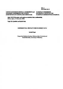
simplicity, each 𝜓𝑖 ∈ Ψ𝑢 can be approximately represented as a (𝑥𝑖 , 𝑦𝑖 , 𝜁𝑖 ), where (𝑥𝑖 , 𝑦𝑖 ) is the location coordinate; 𝜁𝑖 represents the semantic attribute of location coordinate (𝑥𝑖 , 𝑦𝑖 ), i.e., its semantic location. In this way, user’s exposed locations can be transformed into his exposed POIs where he queries LBSs [35]. Indeed, it has been demonstrated that inference of POIs leads to a sever privacy breach [36]. To protect privacy, user usually selects a perturbed POI around him as his real location to request LBSs. Intuitively, to achieve the same level of privacy and LBS accuracy, the perturbed POI should be far more from his real location in a rural area than in downtown. To capture the contextual information in this case, we modify the standard Hilbert curve according to the density of POIs in considering local map and use it to fill the local map (as shown in Figure 3). Figure 3(a) shows the standard Hilbert curve (SHC) that covers the local map. Correspondingly, Figure 3(b) shows the modified Hilbert curve (MHC), which projects every 2dimension POI of users in local map to a 1-d space. Normally, higher density of POIs leads to finer gains such that every point in the 1-dimension space has homogenous context (e.g., equal density). As we will show in the section of location differential perturbation, this prevents a location at a high POIs density area from receiving too large a perturbation to remain utility for LBSs.
Because of the superior distance preserving properties of Hilbert curve that two adjacent points in 1-dimension space are likely to be close in the original space, and vice versa [15], given a particular point, we can easily discover the adjacent points around. With this property, we first project all POIs in considering local map to 1-dimension space by using MHC. Then we randomly perturb the user’s POI where he queries LBS, based on a carefully selected Laplace distribution to guarantee that the probabilities to report the same perturbed POI from a set of likely noise POIs including the true POI are similar. However, the distribution of these noise POIs can affect the proximity of the perturbed POI to the true POI. For instance, if POIs are perturbed based on the locations of every known POI within a city, the scale parameter in the noise distribution will become considerably high, thus leading to heavy noise addition. To solve the problem, we compute the perturbation from a restricted set of k POIs by using the reciprocal framework algorithm [28]. In this way, the probabilities of any POI in these k POIs generating the same perturbed POI are within a small constant factor (up to 𝑒𝜀 ) of each other. Formally, let 𝑙1 , . . . , 𝑙𝑘 represent a set of k noise POIs, one of which is the real POI 𝑙𝑟 =(𝑥𝑟 , 𝑦𝑟 ) of query user, and 𝑝(⋅) indicates the probability density function. For any two POIs 𝑙𝑖 and 𝑙𝑗 in these k noise, the perturbed POI 𝑙𝑝 =(𝑥𝑝 , 𝑦𝑝 )
6
Wireless Communications and Mobile Computing
Input: R as the (rectangle) boundary of the map, Ψ as the set of all POIs in the map Output: a quad-tree root node T (1) if |Ψ| in R is great than pre-determined threshold 𝜎, then (2) partition R equally into four sub-cells Rnw , Rne , Rse , Rsw ; (3) for i=nw, ne, se, sw do (4) return 0 //recursively partition Ri according to the condition |Ψ𝑖 |>𝜎; (5) end for (6) else (7) return 1 //outputs quad-tree root node T; (8) end if Algorithm 1: Modified Hilbert curve construction algorithm.
corresponding to the 𝑙𝑟 is generated in a manner such that 𝑝 (𝑙𝑝 𝑙𝑖 ) ≤ 𝑒𝜀 𝑝 (𝑙𝑝 𝑙𝑗 ) ,
(1)
where 𝜀 > 0 and 𝑖, 𝑗 ∈ [1, 𝑘]. The privacy parameter 𝜀 corresponds to the strength of the privacy guarantee: smaller 𝜀 yield more privacy. It has been shown that adding noise to each coordinate independently (by applying Laplace noise to each coordinate) provides the stronger protection than adding noise to each point independently (by generating 2dimensional noise vector) [37]. Therefore, we use a Laplace distribution with scale b>0 to perturb each coordinate of the 𝑙𝑖 =(𝑥𝑖 , 𝑦𝑖 ) independently such that 𝑝 (𝑥𝑝 | 𝑥𝑖 ) =
1 −|𝑥𝑖 −𝑥𝑝 |/𝑏 , 𝑒 2𝑏
1 𝑝 (𝑦𝑝 | 𝑦𝑖 ) = 𝑒−|𝑦𝑖 −𝑦𝑝 |/𝑏 . 2𝑏
(2)
The amount of noise to be added to each coordinate is given as –b∗sign(rnd)∗ln(1-2|𝑟𝑛𝑑|), where rnd is a uniform random value in (-1/2, 1/2). Based on the following observation, 𝑥𝑝 is generated by setting 𝑏 as (maxn xn -minn xn )/𝜀, and 𝑦𝑝 is generated by setting 𝑏 as (maxn yn -minn yn )/𝜀. 𝑙𝑝 is obtained as (𝑥𝑝 , 𝑦𝑝 ). Observation 1. Using the triangle inequality, we have |𝑙𝑗 −𝑙𝑝 | ≤ |𝑙𝑗 − 𝑙𝑖 | + |𝑙𝑖 − 𝑙𝑝 |. After rearrangement, dividing by b, raising as a power of 𝑒 and multiplying by 1/2b, we get 1 −|𝑙𝑖 −𝑙𝑝 |/𝑏 1 ≤ 𝑒−|𝑙𝑗 −𝑙𝑝 |/𝑏 𝑒|𝑙𝑖 −𝑙𝑗 |/𝑏 𝑒 2𝑏 2𝑏
(3)
𝑜𝑟 𝑝 (𝑙𝑝 | 𝑙𝑖 ) ≤ 𝑝 (𝑙𝑝 | 𝑙𝑗 ) 𝑒|𝑙𝑗 −𝑙𝑖 |/𝑏 . Therefore, for each coordinate, we have 𝑝 (𝑥𝑝 | 𝑥𝑖 ) ≤ 𝑒|𝑥𝑗 −𝑥𝑖 |/𝑏 𝑝 (𝑥𝑝 | 𝑥𝑗 ) , 𝑝 (𝑦𝑝 | 𝑦𝑖 ) ≤ 𝑒|𝑦𝑗 −𝑦𝑖 |/𝑏 𝑝 (𝑦𝑝 | 𝑦𝑗 ) ,
(4)
and the power of the exponent is bounded as 𝑝 (𝑥𝑝 𝑥𝑖 ) ≤ 𝑒|max𝑛 𝑥𝑛 −min𝑛 𝑥𝑛 |/𝑏 𝑝 (𝑥𝑝 𝑥𝑗 ) ,
(5)
𝑝 (𝑦𝑝 𝑦𝑖 ) ≤ 𝑒|max𝑛 𝑦𝑛 −min𝑛 𝑦𝑛 |/𝑏 𝑝 (𝑦𝑝 𝑦𝑗 ) .
(6)
Consequently, the probability of a POI generating a certain perturbed POI is always with a factor 𝑒𝜀 of the probability of some other POIs in the set of k noise generating the same perturbed POI.
4. Location Differential Perturbation In this section, we introduce the modified Hilbert curve construction algorithm and location differential perturbation algorithm in detail. 4.1. Modified Hilbert Curve Filling. Without loss of generality, we consider a set of users U = {𝑢1 , 𝑢2 , . . . , 𝑢𝑛 } who subscribe certain LBSs and move in a local map. The (rectangle) boundary R of the local map is taken as a large cell. We recursively partition a cell into four equal-size cells if and only if the number of POIs within the original cell is greater than a predetermined threshold 𝜎. One can see that each cell contains roughly 𝜎 or fewer POIs. Figure 3(b) depicts an example of such a partition. From the figure, we can see that each cell is either partitioned into four equal-size square cells, or not partitioned (i.e., becoming a base cell). The partitioning scheme can be readily represented as a quadtree. Figure 3(c) depicts an example of such a quad-tree for the MHC mapping in Figure 3(b). In particular, each node in the tree either is a leaf node (if corresponding to a base cell) or contains four children (if further partitioned). Thus, to efficiently store the tree, we construct a breath-first traversal of the tree, storing 1 bit for each node indicating whether it is a leaf node or not. Since a quad-tree with 𝑛 leaf nodes has at most 4n/3 total nodes, the space required by the serialized map file is at most 4n/3 bits. Thus, the total storage overhead is O (n). One can see that MHC covers the regions of high density of POIs with finer gains. Algorithm 1 depicts the offline construction of MHC. In the algorithm, we partition original map based on predetermined threshold parameter 𝜎 (line (1)), recursively partition their children according to the given conditions and store the quad-tree into a bit stream (line (4)). The computational complexity of Algorithm 1 is O (n). After the partitioning process, we construct the mapped 1-d space as variation of the Hilbert space-filling curve [38] to connect all cells in the original 2-d space. To assign a corresponding range in the 1-d space for each base cell, we
Wireless Communications and Mobile Computing
7
Input: the T obtained from Algorithm 1, starting point 𝑆0 and curve orientation 𝜃 Output: a updated quad-tree root node T (1) initializes S(T) = 𝑆0 , 𝜃(T)= 𝜃, m = 0; (2) push T into the stack; (3) while (stack is not empty) do (4) N = pop the top element from the stack (5) if (N has child node) then (6) for (i= sw, se, ne, nw) do (7) set S(Ni ), and 𝜃(Ni ) (8) push Ni into the stack (9) end for (10) else (11) ℎN = m (12) set the values of all corresponding POIs in the node N as m (13) m=m+1 (14) end if (15) end while (16) outputs the updated quad-tree root node T. Algorithm 2: Hilbert value generation algorithm for each base cell.
need to traverse every leaf node. To this end, we conduct a depth-first traversal of tree T, assigning the Hilbert value in the 1-d projected space for each leaf node according to its visiting orders. Let S(N), 𝜃(N) be the orientation and starting point of the Hilbert curve of the node N. The Hilbert value corresponding to the node N is denoted by ℎN . The formal description of our Hilbert value generation algorithm can be found in Algorithm 2. In Algorithm 2, we construct a depth-first traversal over the quad-tree. In particular, we start from the root node T (lines (1)-(2)) and determine its every child node’s curve orientation 𝜃 and starting point 𝑆 in the manner of drilldown according to the fractal rules used in our recent work [39] (lines (7)-(8)). We repeat this process until reaching a leaf node and set the Hilbert value of this leaf node as m (line (11)). In such way, every leaf node is assigned to a unique Hilbert value. Correspondingly, the Hilbert value of all POIs in every leaf node is also obtained (line (12)). The computational complexity of Algorithm 2 is O (n). 4.2. Location Perturbation Algorithm. In Section 3.2, we provide a method to generate a perturbed POI for query point from the carefully selected k POIs by using the Laplace distribution. As mentioned before, the k POIs should be chosen to preserve reciprocity. That is, the same anonymous set should be obtained irrespective of which of the k POIs is the query point. This is achieved by using the reciprocal framework algorithm [28], which partitions the POIs of user into k size buckets based on the Hilbert value of the POIs. The anonymous set is selected as the bucket to which the query point belongs. Each of the k POIs is used for perturbation and the one having the minimum average distance to all POIs in the anonymous set is chosen as the user’s location to issue the query. The formal description of our location perturbation algorithm can be found in Algorithm 3.
In Algorithm 3, we firstly index the all-possible POIs by a quad-tree spatial index and assign the Hilbert value for each POI (Line (1)). This step has time complexity of 𝑂(𝑛). Then we find the mapped value based on the 1-d value range of the base cell which contains 𝜓𝑢 (line (2)). One can see that the retrieval process requires access at most log 𝑛 (the depth of tree) nodes, leading to computational complexity of O(log 𝑛). Based on the Hilbert indices of the POIs, we determine the k size bucket to which the 𝜓𝑢 belongs by using reciprocal framework (lines (3)-(9)), which has time complexity of O(log 𝑛). The locality preserving properties of Hilbert curves guarantee the formation of buckets with POIs that are at close proximity to each other. Lines (10)(14) compute a perturbed value corresponding to the k POIs in the bucket by using Laplace distribution. Thus, each coordinate 𝑐 of a POI is perturbed to c–b∗sign(rnd)∗ln(12|𝑟𝑛𝑑|), where rnd is a uniform random value in (-1/2, 1/2), and 𝑏 is set as (maxn cn -minn cn )/𝜀. This makes perturbation Laplace distributed around 𝑐. In the following experiment, the retrieval of the MHC mapping requires less than 0.1s in our system, and the perturbation requires less than 0.5s. 4.3. Security Analysis. In this section, we provide security analysis. In the context of location privacy, we consider two types of adversaries: active adversary and passive adversary. The purpose of the passive adversary is to obtain sensitive information about a particular user by eavesdropping on the wireless channel or compromising the LBS provider. Actually we can use some cryptography tools such as public key infrastructure (PKI) to cope with the eavesdropping attacks on the wireless channel between users and other entities. Thus, we mainly focus on how to avoid collusion attacks and inference attacks from active adversary, both of which can cause serious privacy problems. Adversary may be collusion with some users or the LBS server to capture the other user’s private information.
8
Wireless Communications and Mobile Computing
Input: Query user 𝑢 with associated k, his POI 𝜓𝑢 where he queries LBSs, and the precomputed MHC filling file mhcFile Output: A perturbed location 𝑙𝑝 for u (1) load a quad-tree T of the partition from mhcFile and use Algorithm 2 to assign the Hilbert value for each POI; (2) find the leaf node N containing 𝜓𝑢 ; (3) while (there is non-empty node at the same level as N with < k POIs) do (4) N = parent of N //bottom-up traversal (5) end while (6) while (N is not a leaf and (each child of N is either empty or contains ≥ k POIs)) do (7) N=child of N that contains 𝜓𝑢 //top-down traversal (8) end while (9) obtain the L={𝑙1 , . . . , 𝑙𝑟 , . . . 𝑙𝑘 } by splitting the POIs inside sub-tree of N into buckets containing between k and 2k-1 POIs using reciprocal algorithm (10) L𝑝 =𝜙 (11) for (𝑙 ∈ L) do (12) 𝑙𝑝 = l + 𝑧𝑖 , where 𝑧𝑖 is additive noise generated by Laplace distribution (13) Lp = Lp ∪ {𝑙𝑝 } (14) end for (15) output 𝑙𝑝 ∈ L𝑝 such that 𝑙𝑝 has minimum average distance from L. Algorithm 3: Location perturbation algorithm.
Theorem 1. Our scheme is collusion attack resistant. Proof. We contemplate that the collusion attack occurs between a set of users. On the one hand, each user is independent with others in our scheme. He only needs to use his position and the stored Hilbert index file to generate the perturbation instead of interacting with the other users. On the other hand, Algorithm 3 in our scheme guarantees that all the processes are executing locally, not dependent on other users at all. That is, it is useless for the adversary to capture and collude with nearby users. The best case to this kind of adversary is that he can obtain the global information by capturing the LBS server and all the users, but in this case he becomes an active adversary to perform inference attack. In our scheme, we directly contemplate the untrusted LBS server as the active adversary to perform the inference attack. He can get side information by monitoring all the users in the system, including their interests, approximately location (e.g., a set of likely positions including the true location), LBS queries, and observed perturbation. His aim is to use this side information to confidently infer real position of the query user. Theorem 2. Our scheme is inference attack resistant under 𝜀differential privacy. Proof. In our scheme, users need to issue the queries to the adversary in order to enjoy the LBSs. Ideally, due to the perturbation, the adversary cannot construct any direct linkage from the perturbed locations to a user. However, the adversary knows the POIs density of the whole map, approximately locations for a user and noise distribution. Based on this information, the adversary can perform inference attacks to gain the real location of the query user. More formally, the adversary knows the set of all POIs, Ψ, a set of positions, 𝑙1 , . . . , 𝑙𝑟 , . . . , 𝑙𝑘 (including query user’s real location), location
perturbation mechanism, and the noise distribution 𝑝(𝑙i ). As certain position in the adversary’s approximate knowledge is highly unlikely to generate the observed perturbation under the used noise distribution, the adversary can use newly learned distribution to improve its probability of successfully guessing the real location from these equally likely positions. In our algorithm, the inference attack is avoided by using reciprocity framework and 𝜀-differential privacy. First, since the k POIs set L={𝑙1 , . . . , 𝑙𝑟 , . . . , 𝑙𝑘 } generated by using MHC method satisfies reciprocity, the probability of identifying the query user’s real POI does not exceed 1/k [28]. Second, as discussed above, due to the usage of differential privacy, the probability to report the same observed perturbed location 𝑙𝑝 from the positions 𝑙1 , . . . , 𝑙𝑟 , . . . 𝑙𝑘 is within a small constant factor of each other. The Laplace noise added to a POI depends on the component-wise maximum distance between two positions. As long as the scale parameters use these maximum, the perturbed POI (𝑥𝑝 , 𝑦𝑝 ) will satisfy the probability ratio. In our scheme, we use differential privacy notion to abstract the side information and guarantee the security efficiently. For any two POIs 𝑙𝑖 and 𝑙𝑗 in the set L, the adversary’s side information can be modelled by two prior distributions 𝑝(𝑙𝑖 ) and 𝑝(𝑙𝑗 ). After observing the perturbed POI 𝑙𝑝 , the adversary could use the 𝑙𝑖 and 𝑙𝑗 as input to differential location perturbation algorithm and compute the conditional probabilities 𝑝(𝑙𝑝 | 𝑙𝑖 ) and 𝑝(𝑙𝑝 | 𝑙𝑗 ). For the purpose of modelling the adversary’s observation, we use Bayes’ rule to obtain the posterior distribution: 𝑝 (𝑙𝑖 = 𝑙𝑟 | 𝑙𝑝 ) = 𝑝 (𝑙𝑗 = 𝑙𝑟 | 𝑙𝑝 ) =
𝑝 (𝑙𝑝 | 𝑙𝑖 ) 𝑝 (𝑙𝑖 ) ∑𝑘𝑐=1
𝑝 (𝑙𝑝 | 𝑙𝑐 ) 𝑝 (𝑙𝑐 )
𝑝 (𝑙𝑝 | 𝑙𝑗 ) 𝑝 (𝑙𝑗 ) ∑𝑘𝑐=1 𝑝 (𝑙𝑝 | 𝑙𝑐 ) 𝑝 (𝑙𝑐 )
, (7) .
Wireless Communications and Mobile Computing
9
We use multiplicative distance to metric the distance between two distributions as 𝑝 (𝑙𝑖 | 𝑙𝑝 ) ≤ 𝜀 𝑑𝑝 = sup ln 𝑝 (𝑙 | 𝑙 ) 𝑙⊆𝐿 𝑗 𝑝
(8)
According to the definition of 𝜀-differential privacy, the 𝑑𝑝 should be at most 𝜀. Substituting formula (7) into formula (8), we can get 𝑝 (𝑙𝑝 | 𝑙𝑖 ) ≤ 𝑒𝑅/𝑏 𝑝 (𝑙𝑝 | 𝑙𝑗 ) ,
lp
(9)
where 𝑅 is the radius of maximum perturbation range which satisfies Laplace distribution, also the maximum distance between any two noise POIs, and 𝑏 is the scale parameter of Laplace distribution. Thus, formula (9) can be extended to formulas (5) and (6). As can be seen from formula (9), our scheme is independent of the prior distribution. This is to say, the probabilities that the adversary uses side information to report the same observed perturbed location 𝑙𝑝 from the positions 𝑙1 , . . . , 𝑙𝑟 , . . . 𝑙𝑘 are within a small constant factor of each other. Thus, the adversary cannot use such side information to improve its probability of successful guessing the real location.
Figure 4: AOI and AOR with centre 𝑙𝑟 and 𝑙𝑝 .
(iii) Displacement: it captures the average difference in distance between the actual results and real retrieval results of a KNN-query, given as 𝑄𝑃 𝐾
4.4. Query Accuracy Analysis. In this section, we provide LBS query accuracy analysis. Using perturbed locations do affect the accuracy of query results. However, difference in the results may or may not exist depending on the distance between the perturbed location and the true location. Therefore, one has to trade-off between location privacy and LBS utility. In order to formally analyze the query accuracy of our location perturbation scheme, we consider three metrics with respect to KNN query [8]: Nearness, Resemblance, and Displacement. (i) Nearness: it indicates the ratio of perturbation at close proximity to the true location. (ii) Resemblance: it depicts the accuracy rate of query results retrieved by a KNN query related to a perturbed location. Let 𝑂 = {𝑜1 , 𝑜2 , ⋅ ⋅ ⋅ , 𝑜𝐾 } be the objects retrieved by a KNN-query relative to the } true location of user u, and 𝑂 = {𝑜1 , 𝑜2 , ⋅ ⋅ ⋅ , 𝑜𝐾 be the objects retrieved relative to the perturbed location. The resemblance is the rate of common objects between 𝑂 and 𝑂 , given as 𝑄𝐴𝑅
𝑂 ∩ 𝑂 , = |𝑂|
lr
(10)
where |𝑂| is the number of query objects in the real results set O, |𝑂 ∩ 𝑂 | is the number of common objects between 𝑂 and 𝑂 .
𝐾
1 { { [∑𝑑𝑖𝑠𝑡 (𝑂𝑖 , 𝑞) − ∑𝑑𝑖𝑠𝑡 (𝑂, 𝑞)] , = { 𝐾 𝑖=1 𝑖=1 { 0, {
𝑂 ≠ 𝑂
(11)
𝑂 = 𝑂 ,
where 𝑞 is the real query POIs of a user and the dist(⋅) is the Euclidean distance between an object’s location and the true location of a user. It should be noted that the lowercase 𝑘 is used to calculate anonymous set and the uppercase 𝐾 is used to calculate KNN query. These three metrics are used to measure the effectiveness of our scheme. The resemblance measures the query accuracy with respect to the perturbed location, while the displacement measures the expected distance error between the real query results and actual retrieval results. In this part of theoretical analysis, we adopt the Resemblance metric as the query accuracy measure. Nevertheless, in the following experimental evaluation, we also evaluate the Nearness and Displacement metrics. As shown in Figure 4, we define the blue circle as the query area of interest (AOI) with regard to the real location 𝑙𝑟 and the orange circle as the area of retrieval (AOR) with respect to the perturbed location 𝑙𝑝 . In order to guarantee high Resemblance (see formula (10)), ideally, the AOR should always completely contain the AOI. Unfortunately, this condition cannot be guaranteed because of the nature of our location perturbation (note that the AOR is centred on a randomly generated location that can be arbitrarily distant from the real location). In order to measure the probability of such event, we introduce the notion of accuracy. Specifically, we use 𝑟𝐼 and 𝑟𝑅 to represent the radius of the AOI and
10
Wireless Communications and Mobile Computing
(b) MHC filling of NA with 𝜎=10
(a) Road network of NA
Figure 5: NA dataset.
the AOR, respectively, M to denote the location perturbation mechanism, and C(x, r) to denote the circle with centre 𝑥 and radius r. Definition 3. An LBS perturbation is (c, 𝑟𝐼 )-accurate iff for all locations 𝑥 we have that C(x, 𝑟𝐼 ) is fully contained in the C(M(x), 𝑟𝑅 ) with probability at least c. Give a privacy parameter 𝜀 and accurate parameters (c, 𝑟𝐼 ), our goal is to obtain an LBS perturbation (M, 𝑟𝑅 ) satisfying both 𝜀-differential privacy and (c, 𝑟𝐼 )-accurate. As for a perturbation mechanism M, we use the Laplace perturbation 𝑀𝜀 discussed in Section 3.2, which satisfies 𝜀differential privacy. As for 𝑟𝑅 , we attempt to find a minimum value validating the accurate condition. To achieve this goal, we use the notion of (𝛼, 𝛿)-usefulness, which was introduced in [40]. A location perturbation mechanism 𝑀 is (𝛼, 𝛿)usefulness if for every location 𝑥 the perturbed location z = M(x) satisfies 𝑑𝑖𝑠𝑡(𝑥, 𝑧) ≤ 𝛼 with probability at least 𝛿. In our perturbation mechanism 𝑀𝜀 , we computer the perturbation from a restricted set of k POIs that preserve reciprocal. This guarantee that our 𝑀𝜀 can generate reasonable perturbation range. Therefore, the 𝛼 and 𝛿 values which express 𝑀𝜀 usefulness are related by –b∗sign(rnd)∗ln(1-2|𝑟𝑛𝑑|), the noise amount of our perturbation. Observation 2. For any 𝛼 > 0, 𝑀𝜀 is (𝛼, 𝛿)-usefulness if 𝛼 < max𝑖,𝑗∈[1,𝑘] 𝑑𝑖𝑠𝑡(𝑙𝑖 , 𝑙𝑗 ), where 𝑙𝑖 and 𝑙𝑗 are determined by –b∗sign(rnd)∗ln(1-2|𝑟𝑛𝑑|). In the following experimental evaluation (as shown in Table 2), we set various 𝜀 to compute the percentage of the perturbations which are within 1km, 0.5km, and 0.1km of the user’s true position. As our running example, our perturbation mechanism 𝑀𝜀 (𝜀-differential privacy, with 𝜀 = 0.5) generates a perturbed location 𝑙𝑝 falling within 1km of the real position 𝑙𝑟 with probability 0.9426.
According to the definition of usefulness, if 𝑀𝜀 is (𝛼, 𝛿)usefulness, then the LBS perturbation (𝑀𝜀 , 𝑟𝑅 ) is (𝛿, 𝑟𝐼 )accurate if 𝛼 < max𝑖,𝑗∈[1,𝑘] 𝑑𝑖𝑠𝑡(𝑙𝑖 , 𝑙𝑗 ). The converse also holds if 𝛿 is maximal. By Observation 2, we have the following. Proposition 4. The LBS perturbation (𝑀𝜀 , 𝑟𝑅 ) is (𝛿, 𝑟𝐼 )accurate if 𝑟𝑅 ≥ 𝑟𝐼 + 𝛿 ⋅ max𝑖,𝑗∈[1,𝑘] 𝑑𝑖𝑠𝑡(𝑙𝑖 , 𝑙𝑗 ). Therefore, it is sufficient to set 𝑟𝑅 = 𝑟𝐼 + 𝛿 ⋅ max𝑖,𝑗∈[1,𝑘] 𝑑𝑖𝑠𝑡(𝑙𝑖 , 𝑙𝑗 ). Thus, our perturbation (𝑀𝜀 , 𝑟𝑅 ) satisfies both 𝜀-differential privacy and (𝛿, 𝑟𝐼 )-accurate.
5. Experimental Evaluation This section evaluates the proposed differential location perturbation algorithms. We implemented the algorithms using Java program. All experiments were executed on an Intel Core i7-4790 3.6GHz machine with 4G RAM and Windows OS. The perturbation scheme indexes the allpossible POIs of the considering local map, which are taken from the NA dataset (available at http://www.cs.utah.edu/∼ lifeifei/SpatialDataset.htm) containing 175813 real POIs of the North America road network (see Figure 5(a)). The parameter k is set from 10 to 1000. The results are obtained by taking the average of 100 times simulation of the corresponding algorithms. Several parameters are employed in our evaluation. 𝑆0 is the starting point of Hilbert curve, and its default value is (0, 0). The 𝜃 represents the Hilbert curve direction, and its default value is D1 (see Figure 6) [39]. Γ is the scale factor of Hilbert curve, and its default value is 1. k is related to k-anonymity. Figure 5(b) shows a real MHC filling for the North America road network with 𝜎=10. From the figure, an intuitive observation is that the denser regions represent large cities, while the sparse regions represent the rural areas. Thus, MHC mapping captures the contextual information well. In [9], Shokri proposes an optimal location privacy preservation strategy by solving a linear program, which avoids TTP.
Wireless Communications and Mobile Computing 1
2
1
0
3
0
3
2
0
3
2
3
2
1
0
1
D1
y
11
R1
U1
L1
2
1
2
3
0
3
0
1
3
0
1
0
1
2
3
2
x
D2
R2
U2
L2
Figure 6: Fractal rules of Hilbert curve.
5.1. Parameters Selection for MHC and SHC. During the partitioning process, MHC and SHC employ different curve parameters. To carry out the following experiments under the same standard, we first examine the parameters selection for MHC and SHC. When the geographic space is filled by using MHC mapping, a unique index value is assigned to each atomic region according to the traversal order of the Hilbert curve. The index values of the POIs contained in the atomic region are also index value of the atomic region. Thus, we can obtain the Hilbert index of all POIs. If some POIs are in the same base cell, they are overlapped. We define the overlap factor 𝜆 to describe the overlap of the POIs for each base cell such that 𝜆=
1 𝐻 ∑𝑛 𝑀 𝑖=0 𝑖
(12)
5 4 3
This optimal strategy computes location obfuscation probability distribution function to maximize the location privacy, subject to service quality constraints. However, this method depends on the modelling of adversary’s side information and thus suffers from background knowledge attacks. As can be seen from previous analysis, our method abstracts adversary’s side information. Furthermore, this optical strategy has nothing to do with contextual information and Hilbert curve. Therefore, our method cannot be comparable to this optical strategy. Location perturbation method in [8] is similar to our approach and uses SHC, whereas it still employs a TTP. For the purpose of comparing with [8], we implement the method in [8] under the same setting as our method. To generate the k-anonymous sets, the location perturbation scheme in [8] employs SHC to calculate the Hilbert index value of users’ location online. Different from the method in [8], our scheme employs MHC to calculate the Hilbert indices of the POIs and stores them as a binary map file. We use the quad-tree recovered from the binary map file to find the node where the user’s POIs are located and then generate the k-anonymous set. Therefore, in the following experiment, we evaluate the performance of the location perturbation by comparing MHC mapping with SHC mapping.
2 1 0
1
2
3
4
5
6
7
8
9
10
Figure 7: The relationship between 𝜎 and 𝜆.
where 𝑀 is the number of base cells that contain POIs, H is the upper bound of the Hilbert index value, and 𝑛𝑖 represents the number of the POIs whose index value is equal to i. Figure 7 illustrates the case that the MHC overlaps factor 𝜆 changes with the division threshold 𝜎. We find that 𝜆 grows slowly as 𝜎 increases, and when 𝜎 is 1, the overlap factor is also 1. This is determined by the definition of the overlap factor and the division in Algorithm 2. The MHC can achieve finer grains via setting the threshold 𝜎. Figure 8 illustrates the relationship between the standard Hilbert curve degree 𝐷 and the overlap factor 𝜆 when the map of the NA dataset is divided by the SHC. As can be seen from the figure, the larger 𝐷 is, the smaller 𝜆 is and the finer grain that the partition leads to. Since the SHC employs the uniform standard to divide the space, the 𝜆 changes greatly with the changing of the 𝐷 when 𝐷 is small. In [8], the SHC mapping technique was employed to divide the entire map into a grid of 214 ∗ 214 while calculating the Hilbert indices, which guarantees that there is not more than one user in each division. Objects in the same division have the same Hilbert index. This is because a larger curve degree 𝐷 can lead to a finer granularity division of spatial maps. Nevertheless, the greater curve degree may lead to high computational overhead unaffordable to the server.
12
Wireless Communications and Mobile Computing Table 1: Hilbert index generation time (ms). 𝜆=1 𝜎=1, D=13 1237 892
Algorithm
SHC MHC
𝜆 = 1.5 𝜎=2, D=11 1067 521
14
1.4
12
1.2 Generation Time (s)
10
𝜆 =2.7 𝜎=5, D=10 988 300
8 6 4 2 0
8
9
10
11 D
12
13
14
𝜆 =4.9 𝜎=10, D=9 903 214
1 0.8 0.6 0.4 0.2 0
Figure 8: The relationship between 𝜆 and D.
2
100
200
300
400
500
600
700
800
900 1000
k
5.2. Anonymous Evaluation. We compare the average anonymous set generation time of our scheme and the scheme in [9] for varying k (see Figure 9). As can be seen from Figure 10, as the 𝑘 increase, the anonymous set generation time for MHC perturbation (see Algorithm 3) and SHC perturbation (see [8]) does not vary significantly. This is because, in both perturbation algorithms, to select the k-anonymous set that satisfies reciprocity we only need to traverse the small subtree determined by node N in the quad-tree T, and the data structure of the intermediate nodes of the quad-tree T contains all the POIs in its subtree, so there is no need to traverse their subtrees to obtain this information. In the case of the same k, the anonymous sets generation time of MHC perturbation is much lower than that of SHC perturbation, with an average reduction about
MHC-Perturbation SHC-Perturbation
Figure 9: Anonymous set generation time for varying k.
Resemblance
The generation time of the index of POIs is an important measure when using the spatial filling curve to divide the considered map. We compare the index generation time of our scheme using MHC padding algorithm HVGA with the scheme using SHC padding algorithm EDHO in [8]. The HVGA represents the Hilbert value generation algorithm (see Algorithm 2). The results are shown in Table 1. As seen from the table, in the case of the same 𝜆, the efficiency of Hilbert index generation via using the MHC mapping technology in our scheme is significantly higher than that via using SHC mapping technology in [8], and with the increase of 𝜆, the result of using MHC is more obvious. This is because the MHC partition considers the density distribution of POIs and uses different curve degree 𝐷 for different density regions, which enable the partitioning of the lower density region not use high D, thus improving the efficiency of index generation. When 𝜎 ≥ 10, the MHC index generation time changes very slowly. Therefore, in all the following experiments we considered the 𝜆 = 4.9, 𝜎 = 10, D = 9.
1.0 0.9 0.8 0.7 0.6 0.5 0.4 0.3 0.2 0.1 0.0
1
2
3
4
5
6
7
8
K MHC-Perturbation SHC-Perturbation
Figure 10: Query accuracy rate of KNN retrieval.
66%. This is because when the location index is generated, the SHC perturbation is partitioned by the uniform granularity for all the regions; nevertheless, the MHC is divided according to the density distribution of the POIs. The MHC partition of the sparse regions uses lower curve orders and thus reduces the division time. That is to say, in the same case, the MHC partition traverses fewer subtrees than the SHC partition. 5.3. Differential Location Perturbation Evaluation. In this section, we evaluate the performance of our differential location perturbation algorithm by comparing MHC mapping with SHC mapping. From Section 3.2, we know that the probability ratio of generating the perturbed position (𝑥𝑝 ,
Wireless Communications and Mobile Computing
13
Table 2: Percentage of the generated perturbed positions that is at close proximity to true location.
0.01 0.1 0.3 0.5 1.0 2.0
Nearness/% d ≤500m 0.95 16.27 61.24 62.20 73.68 91.87
d ≤1000m 2.39 28.2 89.3 94.26 99.04 99.99
𝑦𝑝 ) at any two POIs in the anonymous is bounded as 𝑒𝜀 . The amount of Laplace noise to be added to the position depends on the maximum distance of the corresponding coordinates of the two positions. As long as the Laplace scale parameter 𝑏 uses these maximum distances, the probability ratio of the any two POIs in anonymous set generating a perturbed position (𝑥𝑝 , 𝑦𝑝 ) always satisfies the bounded 𝑒𝜀 . 𝜀 is privacy budget and smaller 𝜀 yields more privacy, but leading to less accuracy. In the following experiment, we evaluate the accuracy of our scheme for a scenario, where we issue a KNN query for nearest POIs. In particular, we use the Nearness, Resemblance, and Displacement metrics to measure LBS accuracy. (1) Nearness: for the Nearness metric, we set the different privacy parameter 𝜀 to calculate the percentage of the perturbations that resulted in the perturbed point being generated within 1000 m, 500 m, and 100 m of the user’s true position. The results are shown in Table 2. As can be seen from the table, a value of 𝜀 = 0.01 indicates that two users should have the same probability (𝑒𝜀 = 1.01) to generate perturbations. This is difficult to achieve most values of k. When the 𝜀 value reaches 0.5 (𝑒0.5 = 1.65), more than 90 percent of the perturbed points are within 1000 meters of the real position. More than 60 percent of the perturbed points are within 500m of the true position. The number of perturbed points increases with increasing of the 𝜀 value. However, higher 𝜀 value reduces the practical significance of the approach. For example, the value of 𝜀 = 2.0 means that a factor of 7 differences in the probability estimates (e2.0 = 7.39) must be accepted. Nonetheless, high nearness values with smaller value of 𝜀 are also possible as well. (2) Resemblance and Displacement: as previously observed in Table 2, about 95% perturbed points fall within 1km of the real position when 𝜀=0.5. Therefore, for the resemblance metric 𝑄𝐴𝑅 and displacement metric 𝑄𝑃 , we set 𝜀 = 0.5 to generate the perturbations in the experiments. Figures 10 and 11 show the evaluation results of the Resemble and Displacement corresponding to different values of K (the number of the nearest neighbour objects retrieved by KNN). From Figure 10, we can see that increasing the number of nearest neighbouring objects to search K enhances the similarities of the result set. As K increases, the query accuracy rate of KNN retrieval varies from around 60 percent to almost 90 percent. This is because that a greater number of retrieved results can be seen as enlarging the search radius, in which case, an object becomes more likely in the KNN
d ≤100m 0.01 8.13 7.18 11.48 27.27 33.97
0.5 0.4 Displacement (km)
𝜀
0.3 0.2 0.1 0.0
1
2
3
4
5
6
7
8
K SHC-Perturbation MHC-Perturbation
Figure 11: Query precision of the approximate KNN search.
set of more number of location-based queries. For example, searching for the nearest theatres from two different locations in a city, we can expect that these two different locations have higher overlap in their list of 10 nearest theatres. The extent of the overlap depends on how proximal the two locations are to each other. Therefore, the noise added to a location is important in this regard. Meanwhile, the retrieval accuracy of a KNN using MHC is increased by an average 15.4% compared with the approach using SHC. This is because the MHC partition considered the density distribution of the POIs, which needs only a small perturbation to achieve a high level of privacy-preserving in a densely populated area. The query precision indicates the average difference in the distance between the actual results and real retrieval results of a KNN-query based on the real location and the perturbed position, which is more effective in measuring the quality of retrieved results. Figure 11 shows the results of the query precision. From Figure 11, we can clearly see that the query precision of a KNN retrieval related to the perturbed location generated by using SHC perturbation varies from about 120m to 350m and that the query precision of a KNN retrieval related to the perturbed location generated by using MHC perturbation is within 50m. This shows that the query precision of a KNN retrieval related to MHC perturbation is smaller than that of a KNN retrieval related to SHC perturbation. The reason is that MHC considers the contextual information of the POIs, thereby resulting in smaller perturbation than
14
Wireless Communications and Mobile Computing
SHC. The results show that the quality of a KNN retrieval results related to MHC perturbation is higher than that of the results related to SHC, which also corresponds with the character that MHC conducts granularity partition of the defined spaces according to density distribution of the POIs.
Province under Grant 1610RJZA056, in part by the Key Laboratory Opening Project of Opto-Technology and Intelligent Control Ministry of Education under Grant KFKT2016-7, and in part by the Youth Science Foundation of Lanzhou Jiaotong University under Grant 2014026.
6. Conclusion
References
Driven by the prosperity of smart mobile devices equipped with GPS, location-based services, as an import part of Green Mobile Communications and Networks (GMCNs), have become very popular recently in almost all business and society domain. Since these services access private position information, location privacy protection mechanisms are mandatory to ensure the user acceptance of such services. The location-based confounding mechanism based on the cloaking area is a wide range of research techniques to achieve location privacy protection, but most of these technologies rely on TTP and assume that the attacker does not have side information, thus easy to cause location privacy disclosure. In this paper, we proposed a context-aware differential location perturbation technique to protect user privacy. Our scheme, the context information of the user’s location is considered in the event of a perturbation, and the attack of the background information can be effectively prevented without depending on any TTP. We use MHC mapping technology to project each 2-d geographic location of the user on the map into 1-d space and combine the 𝑘 anonymous with the differential privacy techniques to randomly disturb the user’s location, and then to submit the perturbation as the user’s real location to the location service provider. In order to solve the limited resources of mobile devices, we use a quad-tree based approach to transform and to store the users’ context to support efficient retrieval and storage. Through the security analysis and experimental evaluation, we can find that our scheme can resist the inference attacks of approximate position knowledge. Using the perturbation position will not significantly improve the attacker’s prior knowledge about the user’s position, so it has strong privacy protection. However, the identification of some unreasonable perturbation is still a problem. In the future work, we will consider abandoning the anonymity sets to address this problem.
[1] M. Ismail, W. Zhuang, E. Serpedin, and K. Qaraqe, “A survey on green mobile networking: From the perspectives of network operators and mobile users,” IEEE Communications Surveys & Tutorials, vol. 17, no. 3, pp. 1535–1556, 2015. [2] X. J. Zhang, X. L. Gui, and Z. D. Wu, “Privacy preservation for location-based services: a survey,” Journal of Software, vol. 26, no. 9, pp. 2373–2395, 2015, (in Chinese with English abstract). [3] M. Gruteser and D. Grunwald, “Anonymous usage of locationbased services through spatial and temporal cloaking,” in Proceedings of the 1st International Conference on Mobile Systems, Applications and Services, MobiSys 2003, pp. 31–42, May 2003. [4] S. Oya, C. Troncoso, and F. P´erez-Gonz´alez, “Back to the drawing board: Revisiting the design of optimal location privacy-preserving mechanisms,” in Proceedings of the 2017 ACM SIGSAC Conference on Computer and Communications Security, pp. 1959–1972, Dallas, Texas, USA, October 2017. [5] X. Pan, J. L. Xu, and X. F. Meng, “Protecting location privacy against location-dependent attacks in mobile services,” IEEE Transactions on Knowledge and Data Engineering, vol. 8, no. 24, pp. 1506–1519, 2012. [6] N. E. Bordenabe, K. Chatzikokolakis, and C. Palamidessi, “Optimal geo-indistinguishable mechanisms for location privacy,” in Proceedings of the 21st ACM Conference on Computer and Communications Security, CCS 2014, pp. 251–262, November 2014. [7] R. Schlegel, C.-Y. Chow, Q. Huang, and D. S. Wong, “Userdefined privacy grid system for continuous location-based services,” IEEE Transactions on Mobile Computing, vol. 14, no. 10, pp. 2158–2172, 2015. [8] R. Dewri, “Local differential perturbations: location privacy under approximate knowledge attackers,” IEEE Transactions on Mobile Computing, vol. 12, no. 12, pp. 2360–2372, 2013. [9] R. Shokri, G. Theodorakopoulos, C. Troncoso, J.-P. Hubaux, and J.-Y. Le Boudec, “Protecting location privacy: Optimal strategy against localization attacks,” in Proceedings of the 2012 ACM Conference on Computer and Communications Security, CCS 2012, pp. 617–626, October 2012. [10] H. Lu, C. S. Jensen, and M. L. Yiu, “Pad: privacy-area aware, dummy-based location privacy in mobile services,” in Proceedings of the Seventh ACM International Workshop on Data Engineering for Wireless and Mobile Access, pp. 16–23, Vancouver, Canada, June 2008. [11] C. Y. Ma, D. K. Yau, N. K. Yip, and N. S. Rao, “Privacy vulnerability of published anonymous mobility trace,” in Proceedings of the 16th Annual International Conference on Mobile Computing and Networking, pp. 186–196, Chicago, IL, USA, 2010. [12] X. Liu, K. Liu, L. Guo, X. Li, and Y. Fang, “A game-theoretic approach for achieving k-anonymity in location based services,” in Proceedings of the 32nd IEEE Conference on Computer Communications (INFOCOM ’13), pp. 2985–2993, IEEE, Turin, Italy, April 2013. [13] B. Niu, Q. Li, X. Zhu, G. Cao, and H. Li, “Achieving k-anonymity in privacy-aware location-based services,” in Proceedings of
Data Availability The data used to support the findings of this study are available from the corresponding author upon request.
Conflicts of Interest The authors declare that they have no conflicts of interest.
Acknowledgments This work was supported in part by the National Natural Science Foundation of China under Grant 61762058, in part by the Scientifically and Technological Project of Gansu
Wireless Communications and Mobile Computing
[14]
[15]
[16]
[17]
[18]
[19]
[20]
[21]
[22]
[23]
[24]
[25]
[26]
[27]
[28]
[29]
the 33rd IEEE Conference on Computer Communications, IEEE INFOCOM 2014, pp. 754–762, Toronto, Canada, May 2014. A. Khoshgozaran, C. Shahabi, and H. Shirani-Mehr, “Location privacy: Going beyond K-anonymity, cloaking and anonymizers,” Knowledge and Information Systems, vol. 3, no. 26, pp. 435– 465, 2011. A. Pingley, W. Yu, N. Zhang, X. Fu, and W. Zhao, “CAP: A context-aware privacy protection system for location-based services,” in Proceedings of the 29th IEEE International Conference on Distributed Computing Systems Workshops (ICDCS ’09), pp. 49–57, Montreal, Canada, June 2009. K. G. Shin, X. Ju, Z. Chen, and X. Hu, “Privacy protection for users of location-based services,” IEEE Wireless Communications Magazine, vol. 19, no. 1, pp. 30–39, 2012. C. Dwork, “Differential privacy,” in Proceedings of the International Colloquium on Automata, languages and Programming, vol. 4052, Springer, Berlin, Germany, 2006. N. Vratonjic, K. Huguenin, V. Bindschaedler, and J.-P. Hubaux, “How others compromise your location privacy: The case of shared public IPs at hotspots,” in Proceedings of the Privacy Enhancing Technologies Symposium – PETS, vol. 7981, pp. 123– 142, 2013. J. Freudiger, R. Shokri, and J. Hubaux, “Evaluating the privacy risk of location-based services,” in Proceedings of the Financial Cryptography and Data Security, pp. 31–46, 2012. A. Machanavajjhala, J. Gehrke, D. Kifer, and M. Venkitasubramaniam, “L-diversity: privacy beyond k-anonymity,” in Proceedings of the 22nd International Conference on Data Engineering (ICDE ’06), pp. 1–12, Atlanta, Ga, USA, April 2006. N. Li, T. Li, and S. Venkatasubramanian, “t-closeness: privacy beyond k-anonymity and l-diversity,” in Proceedings of the 23rd International Conference on Data Engineering, pp. 1–12, Istanbul, Turkey, April 2007. J. Meyerowitz and R. Roy Choudhury, “Hiding stars with fireworks: location privacy through camouflage,” in Proceedings of the 15th Annual ACM International Conference on Mobile Computing and Networking (MobiCom ’09), pp. 345–356, Beijing, China, September 2009. X. Zhang, X. Gui, and F. Tian, “A Framework for measuring query in Location-based Service,” KSII Transactions on Internet and Information Systems, vol. 5, no. 9, pp. 1717–1732, 2015. R. Shokri, G. Theodorakopoulos, J. Boudec, and J. Hubaux, “Quantifying location privacy,” in Proceedings of the IEEE Symposium on Security and Privacy, pp. 247–262, Oakland, CA, USA, 2011. X. Zhang, X. Gui, F. Tian, S. Yu, and J. An, “Privacy quantification model based on the Bayes conditional risk in LocationBased Services,” Tsinghua Science and Technology, vol. 5, no. 19, pp. 452–462, 2014. Y. H. Xiao and X. Li, “Protecting location with dynamic differential privacy under temporal correlations,” in Proceedings of the 22nd ACM SIGSAC Conference on Computer and Communications Security, pp. 1298–1309, 2015. K. Dong, T. Guo, H. Ye, X. Li, and Z. Ling, “On the limitations of existing notions of location privacy,” Future Generation Computer Systems, vol. 86, pp. 1513–1522, 2018. G. Ghinita, K. Zhao, D. Papadias, and P. Kalnis, “A reciprocal framework for spatial K-anonymity,” Information Systems, vol. 3, no. 35, pp. 299–314, 2010. C.-Y. Chow, M. F. Mokbel, and X. Liu, “A peer-to-peer spatial cloaking algorithm for anonymous location-based service,” in
15
[30]
[31]
[32]
[33]
[34]
[35] [36]
[37]
[38]
[39]
[40]
Proceedings of the 14th Annual ACM International Symposium on Advances in Geographic Information Systems (ACM-GIS ’06), pp. 171–178, New York, NY, USA, November 2006. G. Ghinita, P. Kalnis, and S. Skiadopoulos, “MOBIHIDE: A mobilea peer-to-peer system for anonymous location-based queries,” in International Symposium on Spatial and Temporal Databases, vol. 4605, pp. 221–238, Boston, MA, USA, 2007. J. Manweiler, R. Scudellari, and L. P. Cox, “SMILE: Encounterbased trust for mobile social services,” in Proceedings of the 16th ACM Conference on Computer and Communications Security, CCS’09, pp. 246–255, November 2009. G. Ghinita, P. Kalnis, and S. Skiadopoulos, “PRIVE: anonymous location-based queries in distributed mobile systems,” in Proceedings of the 16th International World Wide Web Conference (WWW ’07), pp. 371–380, May 2007. B. Niu, Q. Li, X. Zhu, G. Cao, and H. Li, “Enhancing privacy through caching in location-based services,” in Proceedings of the 34th IEEE Annual Conference on Computer Communications (IEEE INFOCOM ’15), pp. 754–762, IEEE, May 2015. V. Primault, S. B. Mokhtar, C. Lauradoux, and L. Brunie, “Differentially Private Location Privacy in Practice,” 2015, https://arxiv.org/abs/1410.7744?context=cs. X. H. Chen, A. Mizera, and J. Pang, “Quantifying location privacy revisited: preliminary report,” 2014, http://satoss.uni.lu/. S. Gambs, M.-O. Killijian, and M. N. del Prado Cortez, “Show me how you move and I will tell you who you are,” Transactions on Data Privacy, vol. 4, no. 2, pp. 103–126, 2011. K. Jiang, D. Shao, S. Bressan, T. Kister, and K. Tan, “Publishing trajectories with differential privacy guarantees,” in Proceedings of the 25th International Conference on Scientific and Statistical Database Management, pp. 1–12, July 2013. C. Faloutsos and S. Roseman, “Fractals for secondary key retrieval,” in Proceedings of the ACM SIGACT-SIGMODSIGART Symposium on Principles of Database Systems, pp. 247– 252, New York, NY, USA, 1989. F. Tian, X. Gui, J. An, P. Yang, and X. Zhang, “A densitybased space filling curve for location privacy-preserving,” in Proceedings of the 2014 IEEE International Conference on Services Computing (SCC), pp. 131–138, Atlanta, GA, USA, June 2014. A. Blum, K. Ligett, and A. Roth, “A learning theory approach to non-interactive database privacy,” in Proceedings of the Fortieth Annual ACM Symposium on Theory of Computing (STOC ’08), pp. 609–618, ACM, New York, NY, USA, 2008.
International Journal of
Advances in
Rotating Machinery
Engineering Journal of
Hindawi www.hindawi.com
Volume 2018
The Scientific World Journal Hindawi Publishing Corporation http://www.hindawi.com www.hindawi.com
Volume 2018 2013
Multimedia
Journal of
Sensors Hindawi www.hindawi.com
Volume 2018
Hindawi www.hindawi.com
Volume 2018
Hindawi www.hindawi.com
Volume 2018
Journal of
Control Science and Engineering
Advances in
Civil Engineering Hindawi www.hindawi.com
Hindawi www.hindawi.com
Volume 2018
Volume 2018
Submit your manuscripts at www.hindawi.com Journal of
Journal of
Electrical and Computer Engineering
Robotics Hindawi www.hindawi.com
Hindawi www.hindawi.com
Volume 2018
Volume 2018
VLSI Design Advances in OptoElectronics International Journal of
Navigation and Observation Hindawi www.hindawi.com
Volume 2018
Hindawi www.hindawi.com
Hindawi www.hindawi.com
Chemical Engineering Hindawi www.hindawi.com
Volume 2018
Volume 2018
Active and Passive Electronic Components
Antennas and Propagation Hindawi www.hindawi.com
Aerospace Engineering
Hindawi www.hindawi.com
Volume 2018
Hindawi www.hindawi.com
Volume 2018
Volume 2018
International Journal of
International Journal of
International Journal of
Modelling & Simulation in Engineering
Volume 2018
Hindawi www.hindawi.com
Volume 2018
Shock and Vibration Hindawi www.hindawi.com
Volume 2018
Advances in
Acoustics and Vibration Hindawi www.hindawi.com
Volume 2018