Given a set of points {xt}N t=1 on some affine ... With a sufficient number of points (⥠D â d + 1) and no noise, PCA will .... typically using non convex clustering methods such as k- ... For visualization purposes, a rotation of 180⦠was applied to some of ..... finis dordre un, et la resolution par penalisation-dualite dune classe.
A Convex Approach to Subspace Clustering Henrik Ohlsson and Lennart Ljung
Abstract— The identification of multiple affine subspaces from a set of data is of interest in fields such as system identification, data compression, image processing and signal processing and in the literature referred to as subspace clustering. If the origin of each sample would be known, the problem would be trivially solved by applying principal component analysis to samples originated from the same subspace. Now, not knowing what samples that originates from what subspace, the problem becomes considerably more difficult. We present a novel convex formulation for subspace clustering. The proposed method takes the shape of a least-squares problem with sum-of-norms regularization over optimization parameter differences, a generalization of the `1 -regularization. The regularization constant is used to trade off fit and the identified number of affine subspaces.
I. INTRODUCTION Principal Component Analysis (PCA, [22], [15], also referred to as the Karhunen-Loeve transform) is a fundamental tool in areas such as image and signal processing and maybe the most commonly used method for data analysis. PCA finds the linear subspace that maximizes the variance of the projected samples. It can also be shown that this is the linear subspace which minimizes the sum of squared distances between the samples and the projections. In a least squares sense, the projection onto the m dimensional linear subspace given by PCA is therefore the closest m dimensional description of the samples. This is of course a useful property if one seeks a low-dimensional representation of a set of data and the reason for PCA’s popularity as a compression method. PCA assumes that the data is confined to, or in the vicinity of, a single subspace. Now, if data originates from multiple linear subspaces, PCA will not give a satisfying result. The problem also becomes considerably more complex since it is not known what samples that originates from what subspace. If the origin of each sample would be known, the problem would be trivially solved by PCA. We hence need to estimate the subspaces and decide the origin of samples simultaneously. Methods dealing with the estimation of multiple subspaces are in the literature referred to as subspace clustering methods. For an excellent recent survey of subspace clustering see [28]. Subspace clustering methods can be divided into algebraic methods, iterative methods, statistical methods and spectral clustering methods. Most subspace clustering methods (see e.g., [28]) require a careful initialization. The main reason being that most subspace clustering methods lead to non H. Ohlsson and L. Ljung are with the Division of Automatic Control, Department of Electrical Engineering, Link¨oping University, Sweden, {ohlsson,ljung}@isy.liu.se.
convex optimization problems and can get stuck in local optima leading to poor solutions. This paper presents a novel approach to subspace clustering. The proposed method resembles in a convex optimization problem with a performance that is comparable to state of the art subspace clustering methods (when they manage to find a “good” solution and not get stuck in a “bad” local optima). II. P ROBLEM F ORMULATION An affine subspace can be defined as the set of points S = {x ∈ RD : bT (x + µ) = 0, b ∈ RD×d , µ ∈ RD }. (1) The d columns of b span the orthogonal space S ⊥ . For example, if D = 3, d = 1 and µ = 0, b is the normal to a 2dimensional linear subspace. Given a set of points {xt }N t=1 on some affine subspace, PCA can be used to estimate b. With a sufficient number of points (≥ D − d + 1) and no noise, PCA will recover the true b. Now, consider a data set {xt }N t=1 sampled from n affine subspaces. That is, {xt }N satisfy t=1 xj ∈
n [
Si ,
j = 1, . . . , N,
(2a)
i
with Si ={x ∈ RD : bTi (x + µi ) = 0, bi ∈ RD×di , µi ∈ RD }, (2b) for i = 1, . . . , n. If the origin of each of the samples {xt }N t=1 was known i.e., if the function c(·) such that xj ∈ Sc(j) , j = 1, . . . , N was known, PCA could be applied to identify bi by applying PCA to {xt }t:c(t)=i . With c(·) unknown, the problem becomes considerably more difficult. One then has to, simultaneously, identify to what subspace a sample belongs and at the same time estimate b and µ of the subspaces. Note that PCA would not do any good on this data set. The later, when nor the subspaces or the origin of the samples are known, is referred to as subspace clustering and the topic of this paper. Remark 1 (Noisy data): Data are seldom situated on a low number of affine subspaces but rather in a vicinity of a low number of affine subspaces. (2) will therefore never be satisfied for other than n ≥ N/(D − d + 1) in reality. This is handled in PCA by seeking the linear subspace that minimizes the sum of squared distances between the samples and the projections of the samples onto the subspace.
III. P REVIOUS W ORK As stated in the introduction, subspace clustering methods can be divided into algebraic, iterative, statistical and spectral clustering methods. Algebraic methods use algebraic properties of the unions of subspaces. Of rather recent date, compared to PCA, is the algebraic method Generalized Principal Component Analysis (GPCA, [30], [31]). GPCA has the ability to identify Snmultiple affine subspaces and is built around the fact that i Si can be rewritten as n n [ Y D Si = {x ∈ R : bTi (x + µi ) = 0}. (3) i
i
The coefficients of the n-degree polynomial equation system given by n Y
bTi (xt + µi ) = 0,
t = 1, . . . , N,
(4)
i
can easily be found (assuming {xt }N t=1 are given noise free data on n affine subspaces and N large enough). However, in order to recover the subspaces, we also need to compute the gradient w.r.t. x of this polynomial, ∇x
n Y
bTi (x + µi ) =
n X
i
j
bTj
n Y
bTi (x + µi ).
(5)
i:i6=j
0 Evaluated at any x0 ∈ {xt }N t=1 , say that x belongs to subspace k, gives n n Y Y T ∇x bTi (x + µi ) = b bTi (x0 + µi ). (6) k 0 i
x=x
i:i6=k
If di = 1, i = 1, . . . , n, the right hand side is a scaled version of the vector bk (and can be evaluated using the solution of (4)). The right hand side therefore Qn span the orthogonal space to Sk and if we define ¯bk = bTk i:i6=k bTi (x0 +µi ), the sought Sk is given by Sk = {x ∈ RD : ¯bTk (x + µk ) = 0}. GPCA proceeds by evaluating (6) at new samples x0 ∈ {xt }N t=1 until all subspaces have been recovered. GPCA has attained quite some interest since its introduction and has been applied to a number of applications, e.g., hybrid system identification [32], image processing and segmentation [29], [14]. Since GPCA does not make any assumption concerning the distribution of the data on the subspaces, GPCA does not give a maximum likelihood estimate of the subspace parameters. GPCA works very well in low-noise problems but runs into problems, to estimate e.g., µ, when data become noisy (see e.g., [8], [28]). Iterative methods start by an initial guess for the bmatrices. They then continue in an iterative manner by assigning samples to the closest subspace (estimated in the previous step) and then re-estimate b’s from the samples assign to the subspace. Many variants of this idea exist [2], [27]. The main advantage of this type of methods is their simplicity. However, just like k-means clustering (using Lloyd’s algorithm [18]), iterative methods for subspace clustering are known to be sensitive to initialization.
Statistical methods are based on a model for the data in subspace i of the form x = Ai s + ai + ε,
s ∼ N (0, I), ε ∼ N (0, σi2 I).
(7)
To find the maximum likelihood solution for {Ai } and {ai }, the Expectation Maximization Algorithm (EM, [5]) is often used. Statistical methods for subspace clustering are also known to be sensitive to initialization. Finally, spectral clustering methods. For this type of method, an affinity matrix or similarity matrix is a central concept. The entry ij in this N × N matrix is desired to be 1 if xi and xj belong to the same subspace and otherwise small. Spectral clustering methods proceed by seeking for clusters in the set of eigenvectors to the affinity matrix, typically using non convex clustering methods such as kmeans clustering (see e.g., [28]). For a more detailed discussion on algebraic, iterative, statistical and spectral clustering methods, see [28]. In the following we will take an optimization approach to the subspace clustering problem. Something that will be used is a concept called regularization. Regularization has gained a lot of publicity through methods such as the lasso method [26] and Compressed Sensing (CS, [6], [4]). Both these methods use a `1 -regularization to find sparse solutions. A slightly more general type of regularization is the sum-of-norms regularization. In a statistical linear regression framework, sum-of-norms regularization is called group-lasso [33], since it results in estimates in which many groups of variables are zero. Sum-of-norms regularization has previously been applied to the identification of segmented ARX models [21], piecewise affine systems [20] and to clustering [16]. IV. S UBSPACE C LUSTERING T HROUGH OVERPARAMETRIZATION AND S UM - OF -N ORMS R EGULARIZATION Consider the case where b ∈ RD×1 and n = 1. Let {xt }N t=1 be a set of data situated on a D − 1-dimensional linear subspace. Let b0 be the true b-vector. To find the linear subspace, we could consider the convex optimization problem N X kbT xt k22 , s.t. aT b = 1. (8) min b
t=1
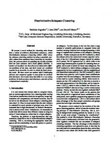
This optimization will perfectly recover the linear subspace 0 if a is such that aT b0 6= 0. To see this, let ¯b be aTb b0 , note that ¯bT xt = 0, t = 1, . . . , N, and that aT ¯b = 1. ¯b is hence the solution to (8). In practice, a can be sampled from a D-dimensional unit Gaussian distribution, making the probability that aT b0 = 0 equal to zero. Example 1 (Comparison to PCA): To examine the ability of the convex formulation (8) to recover the linear subspace of a set of data, we let � � 0 b0 = (9) 1 and sample 100 data points from � � 1 s + ε, s ∼ U (−0.5, 0.5), ε ∼ N (0, 0.01I). 0
(10)
0.8
0.8
0.6
0.6
0.4
0.4
0.2
0.2
x[2]
x[2]
The data is shown with black dots in the left plot of Figure 1. PCA and (6) (a in (6) was sampled from a unit Gaussian) were now applied to the data to get an estimate of b0 . The left plot of Figure 1 shows the b0 -estimates from PCA with dashed line and that of (6) with solid line. Since the data has been disturbed off the one dimensional linear subspace by noise, neither PCA nor (6) give the true b0 . However, we see that the convex optimization approach to estimate b0 (6) is doing fairly well. In the right plot of Figure 1, the resulting estimates and data from 100 runs have been plotted on top of each other (new x’s and a new a in each run).
0
0
−0.2
−0.2
−0.4
−0.4
−0.6
−0.6
−0.8 −0.8
−0.6
−0.4
−0.2
0
x[1]
0.2
0.4
0.6
0.8
−0.8 −0.8
−0.6
−0.4
−0.2
0
0.2
0.4
0.6
0.8
x[1]
Fig. 1. Left plot: Data shown with black dots, estimate of b0 given by PCA showed using dashed line and by (6) by solid black line. Right plot: The same as in the left plot but the result from 100 runs plotted on top of each other. For visualization purposes, a rotation of 180◦ was applied to some of the b-estimates so that the PCA estimate are all between 180◦ and 360◦ and the estimate from (6) between 0◦ and 180◦ .
Remark 2 (Convex optimization formulations of PCA): (6) has the advantage of being a convex optimization problem. Some convex optimization formulations of PCA has been proposed in the literature [24], [25], [3]. We do not believe that (6) can perform better than these but the simplicity made (6) an attractive approach for what is coming. However, any of the methods developed in [24], [25], [3] could potentially also be used in the coming derivations. This has not been exploited. Remark 3 (Subspace of less dimensions than D − 1): Let say that {xt }N t=1 is a set of data situated on a linear subspace of less dimension that D − 1. b0 is then a matrix. If we still seek a b ∈ RD×1 by (6), the found b will be in the orthogonal space to the linear subspace that the data is in (as long as aT b0 6= 0). Having found the D − 1-dimensional subspace containing the data, (6) could now be applied in this D − 1-dimensional space to find the D − 2-dimensional space containing the data, and so on. One could continue this procedure as long as the sum of squared distances between the samples and the projections of the samples onto the subspace is below some threshold. We now turn to the considerably more difficult problem of identifying multiple linear subspaces from a set of samples {xt }N t=1 . Assume for now that the µ’s are zero i.e., we consider linear subspaces. Also, we will assume that subspaces are D−1-dimensional. Subspaces of lower dimension can be handled as discussed in Remark 3 and not further discussed. Since it is unknown what sample that originates from what subspace, we overparametrize and estimate a parameter b for
each sample. To avoid a severe over fit, a regularization that aims at making b’s identical if there is “no need” for them to be different is used. We denote the b associated with xj with bj . The proposed criterion now takes the form
min
bj ,j=1,...,N
N X
k(bj )T xj k22 + λ
j=1
N X
k(xk , xl )kbk − bl k2 ,
k,l=1 T j
s.t. a b = 1, j = 1, . . . , N
(11)
k(·, ·) : RD × RD → R+ is a kernel. This kernel can be used to introduce prior information and should ideally be positive if xk and xl belongs to the same subspace and 0 otherwise. Also in spectral clustering-based methods, this type of similarity kernel is used and there is therefore a whole literature on how to find k(·, ·), see e.g., [7], [17], [28] for interesting choices. The first term in the objective of (11) can be seen as a fit term and the second a regularization. The fit term will be zero if (bj )T xj = 0, j = 1, . . . , N , that is, if bj is orthogonal to xj for all j = 1, . . . , N . Note that as long as aT xj 6= 0, j = 1, . . . , N , there is bj , j = 1, . . . , N, that makes the fit term equal to zero and satisfies the constraint aT bj = 1, j = 1, . . . , N (also for noisy data). The vector a ∈ RD is in the coming assumed sampled from a unit Gaussian. The regularization term is a Sum-Of-Norms regularization (SON regularization). Note that there is no square on the norm in the regularization, this is hence not a sum of squared norms. Sum-of-norms regularization is a well known sparsity regularization, see e.g., [33]. Hence, at the optimum, several of the terms kbi − bj k2 will (typically) be exactly zero. Equivalently, several of the {bj }N j=1 will be identical, and associated x’s can be seen as belonging to the same linear subspace. Remark 4 (Sum-of-norms regularization): The SON regularization used in (11) is an `1 -regularization of the 2-norm of differences bk −bl , k, l = 1, . . . , N . That is, the SON term is the `1 -norm of the vector obtained by stacking kbk − bl k2 , for k, l = 1, . . . , N . Hence, this stacked vector, and not the individual b-vectors, will become sparse. The regularization parameter λ > 0 is a parameter that will control the tradeoff between fit and the number of subspaces. This parameter can be chosen by considering how the sum of squared distances between the samples and the projections of the samples onto the subspaces changes with λ. We will use this in the coming examples to choose λ. Another key property of the proposed criterion for subspace clustering is that the criterion (11) is convex. That means that the global optimum can be found independently of initialization. Many existing subspace clustering methods are dependent of a good initialization for a good result (see e.g., [28]). The convexity also implies that convex constraints easily can be added. The estimated b’s of (11) will be biased due to the regularizatioon and to obtain unbiased estimates, PCA is applied to x’s having the same b’s.
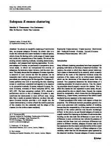
with s sampled from a uniform distribution, s ∼ U (−0.5, 0.5), α = 1 with probability 0.5 and 0 with probability 0.5, ε ∼ N (0, 0.0049I) and � � � � −1 −1 b01 = , b02 = . (13) −0.5 0.5 The data is shown in Figure 2. Motivated by the discussion following (11), we chose k(xk , xl ) = e
|xT k xl | 0.2kxk kkxl k
.
(14)
Now apply (11) for a number of λ’s, see Figure 3. As seen, the sum of squared differences is rather flat for λ < 0.002, indicating that two subspaces (two distinct values in the estimated {bj , j = 1 . . . , N }) is a good choice. We chose λ = 0.001. The members of the two groups are visualized in Figure 2 by the use of a ’o’-symbol for members of the first group and a ’*’-symbol for members of the second group. The resulting estimates of b01 after using PCA on the x’s of the first group is given by a dashed line in Figure 2. The solid line in Figure 2 gives the estimate of b02 obtained by using PCA on the x’s of the second group.
9
# subspaces (−−) & sum of squared differnces between projections and samples (−)
Example 2 (Multiple Linear Subspaces): Let n = 2, D = 2, d = 1 and sample 120 samples from � (12) α(b01 )⊥ + (1 − α)(b02 )⊥ s + ε,
8
7
6
5
4
3
2
1
0
0
0.5
λ
2
2.5
3 −3
x 10
machine. Over 10 runs, no samples were associated with the wrong subspace and the number of subspace were correctly found. So far we have only discussed multiple linear subspaces. Its however straight forward to also handle affine subspaces by a small modification of (11). For affine subspace we propose to consider min j
bj ,µ ,j=1,...,N 0.4
x[2]
1.5
Fig. 3. The number of distinct b’s (or estimated # of subspaces, dashed line) and the sum of squared distances between the samples and the projections of the samples onto the subspaces (solid line) as a function of λ.
0.6
+λ
0.2
1
N X
j T
(b ) xj − µj 2 2 j=1 N X
� k� � l�
µ µ
k(xk , xl )
bk − bl , 2
(15)
k,l=1 T j
s.t. a b = 1, j = 1, . . . , N.
0
−0.2
−0.4
−0.6 −0.6
−0.4
−0.2
0
0.2
0.4
0.6
x[1]
Fig. 2. Data showed with ’*’ and ’o’-symbols. The ’*’-marked data got the same b-estimate using the criterion (11). The ’o’-marked data also got the same b-value but a different value than that of the ’*’-marked data. The PCA-estimate of the true b obtained by applying PCA to either the ’*’ or the ’o’-marked data is also shown using a solid and dashed line.
Example 3 (Larger D, n and N ): To demonstrate that the proposed method (11) is also practical to use on larger problems, the same λ and kernel as in the previous example was used (a threshold was however applied to set k(xk , xl ) to zero if not large enough) on a data set with 40 samples from 10 99-dimensional linear subspaces in 100 dimensions. That is D = 100, n = 10, N = 400 and d = 1. The true b’s were generated by sampling from a zero mean Gaussian distribution. Data was made noisy by adding zero mean Gaussian noise with a variance of 0.25. One simulation (see also Section IV-A) took ∼ 4 minutes on a standard desktop
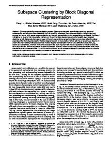
Example 4 (Multiple Affine Subspaces): Let n = 3, D = 2, d = 1 and sample 120 samples from 0 ⊥ α(b1 ) s + µ1 + ε, with probability 1/3, (16) α(b02 )⊥ s + µ2 + ε, with probability 1/3, 0 ⊥ α(b3 ) s + µ3 + ε, with probability 1/3, with s ∼ U (−0.5, 0.5), ε ∼ N (0, 0.004I) and � � � � � � 0 −1 −1 b01 = , b02 = , b03 = , 1 −0.5 0.5 � � � � � � 0 0 0 µ1 = , µ2 = , µ3 = . −0.7 0 0
(17) (18)
We now apply (15) with k(xk , xl ) = e
−
kxk −xl k2 0.15
|xT xl | k kkxl k
+ 0.15kxk
(19)
and for a number of different λ’s, see Figure 5. As seen, the sum of squared differences is rather flat for λ < 2, indicating that four subspaces is a good choice. λ = 0.2 was therefore chosen. The data associated with the first group is visualized with ’*’-symbols in Figure 4. Data associated with the second group, with ’o’ and so on. The resulting estimates after having applied PCA to the data of each group is also
V. C OMPARISON WITH C ONVENTIONAL S UBSPACE C LUSTERING M ETHODS
showed in Figure 4. As seen, one of the three affine subspaces has been divided into two. This could possibly have been avoided by a better choice of kernel k.
In this section we apply generalized PCA with polynomial differentiation and spectral clustering (see [28], Sect. 2.4) and sparse subspace clustering [7] using implementations1 kindly provided by the Vision Lab at Johns Hopkins University. The same data that was used in Examples 2 and 4 were used. GPCA with polynomial differentiation and spectral clustering (using homogeneous coordinates, see [28], and the default for the input parameters) was first applied. The data used in Example 2 resulted in the same plot as Figure 2 and hence an identical result to that of the proposed approach. The data used in Example 4 resulted in the left plot of Figure 6 (cf. Figure 4). Generalized PCA with polynomial differentiation and spectral clustering has some problems finding the true subspaces that the data belongs to but it does a fairly good job in finding the b’s and µ’s. Also sparse subspace clustering (λ = 0.001) recover a result identical to that of the proposed method for the data of Example 2. Data used in Example 4 resulted in the right plot of Figure 6 (cf. Figure 4). As seen, sparse subspace clustering has some problems to recover the affine subspaces. λ = 0.0001 gave the best result in sparse subspace clustering and was used in the right plot of Figure 6.
0.6
0.4
0.2
−0.2
−0.4
−0.6
−0.8
−1 −0.8
−0.6
−0.4
−0.2
0
0.2
0.4
0.6
0.8
x[1]
Fig. 4. Data sampled with noise from three affine subspaces. (15) groups the optimization variables into four groups. The associated points of different groups are shown with different symbols while points of the same group with the same symbol. The figure also shows the computed estimates of the b’s and the µ’s.
9
0.6
0.6
8
0.4
0.4
0.2
0.2
0
0
7
6 x[2]
# subspaces (−−) & sum of squared differnces between projections and samples (−)
10
x[2]
x[2]
0
−0.2
−0.2
5 −0.4
−0.4
−0.6
−0.6
−0.8
−0.8
4
3
2
−1 −0.8
−0.6
−0.4
−0.2
0
0.2
0.4
0.6
0.8
−1 −0.8
−0.6
−0.4
x[1]
−0.2
0
0.2
0.4
0.6
0.8
x[1]
1
0
0
1
2
3
4
λ
5
6
7
8
Fig. 5. The number of distinct b’s (or estimated # of subspaces, dashed line) and the sum of squared distances between the samples and the projections of the samples onto the subspaces (solid line) as a function of λ.
A. Solution Algorithms and Software Many standard methods of convex optimization can be used to solve the problem (11) and (15). Systems such as CVX [13], [12] or YALMIP [19] can readily handle the sumof-norms regularization, by converting the problem to a cone problem and calling a standard interior-point method. Recently, many authors have developed fast, first order methods for solving `1 regularized problems, and these methods can be extended to handle the sum-of-norms regularization used here; see, for example, [23, §2.2]. The simulations shown in this paper was carried out in M ATLAB using CVX. A codepackage for solving (11) and (15) using CVX will be made available for download on http://www.control.isy. liu.se/˜ohlsson/code.html.
Fig. 6. Data sampled with noise from three affine subspaces. The results should be compared to those shown in Figure 4. Left plot: Results using generalized PCA with polynomial differentiation and spectral clustering. Right plot: Results using sparse subspace clustering.
VI. E XTENSIONS Many subspace clustering methods can be extended to handle the identification of hybrid systems and so also the proposed scheme. In fact, it has been shown [20] that the criterion � � 2 N N X X
yk − θkT xk +λ min k(xk , xj )kθk −θj kp
1 2 θk , k=1,...,N k=1
k,j=1
(20) is very suitable for the identification of piecewise affine systems. y is here the measured output of a hybrid system and x the regressor. The θ’s are the sought system parameters associated with the different subsystems. Since {yk }N k=1 now hinders the optimization variables θk from becoming 1 http://www.vision.jhu.edu/gpca.htm, code version: April 19th, 2010 for GPCA with polynomial differentiation and spectral clustering.
identical to zero, a constraint like in (11) and (15) is not needed. See [20] for details. The proposed framework could also be used to estimate nonlinear surfaces or manifolds using kernelization techniques developed in [9]. VII. CONCLUSIONS AND FUTURE WORKS This paper presents a novel intuitive method to subspace clustering. The formulation takes the form of a convex optimization problem and does hence not need a careful initialized, like many other subspace clustering methods. The regularization parameter regulates the number of subspaces identified and is relatively easy to find a good value for. The similarity kernel can be used to introduce prior information. The method’s simplicity together with that it performs well in comparison to state of the art subspace clustering methods should make the method into an attractive choice. A proper evaluation on large scale real data sets is important and something that is to be done. For this purpose, an implementation using Alternating Direction Method of Multipliers (ADMM, [10], [11], see also [1]) is in preparation. Some convex optimization formulations of PCA have been proposed in the literature [24], [25], [3]. These could potentially be used to develop subspace clustering methods in a very similar way as presented in this paper. This has not been exploited but seen as interesting future work. VIII. ACKNOWLEDGMENTS Partially supported by the Swedish foundation for strategic research in the center MOVIII and by the Swedish Research Council in the Linnaeus center CADICS. Also partial support from the European Research Council under the advanced grant LEARN, contract 267381, which is gratefully acknowledged. R EFERENCES [1] S. Boyd, N. Parikh, E. Chu, B. Peleato, and J. Eckstein. Distributed optimization and statistical learning via the alternating direction method of multipliers. Technical report, Stanford University, January 2011. [2] P.S. Bradley and O.L. Mangasarian. k-plane clustering. Journal of Global Optimization, 16:23–32, 2000. [3] E. J. Candes, X. Li, Y. Ma, and J. Wright. Robust Principal Component Analysis? ArXiv e-prints, December 2009. [4] E. J. Cand`es, J. Romberg, and T. Tao. Robust uncertainty principles: Exact signal reconstruction from highly incomplete frequency information. IEEE Transactions on Information Theory, 52:489–509, February 2006. [5] A. P. Dempster, N. M. Laird, and D. B. Rubin. Maximum likelihood from incomplete data via the EM algorithm. Journal of the Royal Statistical Society. Series B (Methodological), 39(1):1–38, 1977. [6] D. L. Donoho. Compressed sensing. IEEE Transactions on Information Theory, 52(4):1289–1306, April 2006. [7] E. Elhamifar and R. Vidal. Sparse subspace clustering. In IEEE Computer Society Conference on Computer Vision and Pattern Recognition, pages 2790–2797, Los Alamitos, CA, USA, 2009. IEEE Computer Society. [8] F. Fabien Lauer, G. Bloch, and R. Vidal. A continuous optimization framework for hybrid system identification. Automatica, 47(3):608– 613, 2011. [9] T. Falck, H. Ohlsson, L. Ljung, J. A.K. Suykens, and B. De Moor. Segmentation of times series from nonlinear dynamical systems. In Proceedings of the 18th IFAC World Congress, Milan, Italy, 2011. To appear. [10] D. Gabay and B. Mercier. A dual algorithm for the solution of nonlinear variational problems via finite element approximation. Computers & Mathematics with Applications, 2(1):17–40, 1976.
[11] R. Glowinski and A. Marrocco. Sur lapproximation par elements finis dordre un, et la resolution par penalisation-dualite dune classe de problemes de Dirichlet nonlineaires. Rev. Francaise dAut., pages 41–76, 1975. Inf. Rech. Oper., R-2. [12] M. Grant and S. Boyd. Graph implementations for nonsmooth convex programs. In V. D. Blondel, S. Boyd, and H. Kimura, editors, Recent Advances in Learning and Control, Lecture Notes in Control and Information Sciences, pages 95–110. Springer-Verlag Limited, 2008. http://stanford.edu/˜boyd/graph_dcp.html. [13] M. Grant and S. Boyd. CVX: Matlab software for disciplined convex programming, version 1.21. http://cvxr.com/cvx, August 2010. [14] W. Hong, J. Wright, K. Huang, and Y. Ma. A multi-scale hybrid linear model for lossy image representation. In IEEE International Conference on Computer Vision, volume 1, pages 764–771, Los Alamitos, CA, USA, 2005. IEEE Computer Society. [15] H. Hotelling. Analysis of a complex of statistical variables into principal components. Journal of Educational Psychology, 24(7):498– 520, 1933. [16] F. Lindsten, H. Ohlsson, and L. Ljung. Clustering using sum-of-norms regularization; with application to particle filter output computation. In IEEE International Workshop on Statistical Signal Processing 2011 (SSP’11), Nice, France, June 2011. To appear. [17] G. Liu, Z. Lin, and Y. Yu. Robust subspace segmentation by low-rank representation. In 27th International Conference in Machine learning (ICML’10), pages 663–670, Haifa, Israel, 2010. [18] S. Lloyd. Least squares quantization in PCM. IEEE Transactions on Information Theory, 28(2):129–137, March 1982. [19] J. L¨ofberg. Yalmip : A toolbox for modeling and optimization in MATLAB. In Proceedings of the CACSD Conference, Taipei, Taiwan, 2004. [20] H. Ohlsson and L. Ljung. Piecewise affine system identification using sum-of-norms regularization. In Proceedings of the 18th IFAC World Congress, Milan, Italy, 2011. To appear. [21] H. Ohlsson, L. Ljung, and S. Boyd. Segmentation of ARX-models using sum-of-norms regularization. Automatica, 46(6):1107–1111, 2010. [22] K. Pearson. On lines and planes of closest fit to systems of points in space. Philosophical Magazine, 2(6):559–572, 1901. [23] J. Roll. Piecewise linear solution paths with application to direct weight optimization. Automatica, 44:2745–2753, 2008. [24] J.A.K. Suykens, T. Van Gestel, J. Vandewalle, and B. De Moor. A support vector machine formulation to PCA analysis and its kernel version. IEEE Transactions on Neural Networks, 14(2):447–450, March 2003. [25] Q. Tao, G.-W. Wu, and J. Wang. Learning linear PCA with convex semi-definite programming. Pattern Recognition, 40(10):2633–2640, 2007. [26] R. Tibsharani. Regression shrinkage and selection via the lasso. Journal of Royal Statistical Society B (Methodological), 58(1):267– 288, 1996. [27] P. Tseng. Nearest q-flat to m points. Journal of Optimization Theory and Applications, 105:249–252, 2000. [28] R. Vidal. Subspace clustering. IEEE Signal Processing Magazine, 28(2):52–68, March 2011. [29] R. Vidal and R. Hartley. Motion segmentation with missing data using power factorization and GPCA. In Proceedings of the 2004 IEEE Computer Society Conference on Computer Vision and Pattern Recognition (CVPR’04), pages 310–316, Washington, DC, USA, 2004. [30] R. Vidal, Y. Ma, and S. Sastry. Generalized principal component analysis (GPCA). In Proceedings of the 2003 IEEE Computer Society Conference on Computer Vision and Pattern Recognition (CVPR’03), pages 1063–1069, June 2003. [31] R. Vidal, Y. Ma, and S. Sastry. Generalized principal component analysis (GPCA). IEEE Transactions on Pattern Analysis and Machine Intelligence, 27(12):1945–1959, December 2005. [32] R. Vidal, S. Soatto, Y. Ma, and S. Sastry. An algebraic geometric approach to the identification of a class of linear hybrid systems. In Proceedings of the 42nd IEEE Conference on Decision and Control (CDC), volume 1, pages 167–172, Hawaii, USA, December 2003. [33] M. Yuan and Y. Lin. Model selection and estimation in regression with grouped variables. Journal of the Royal Statistical Society, Series B, 68:49–67, 2006.