Disease Awareness in Social Networks ... investment on disease awareness throughout the network when the cost function ..... largest eigenvalue is λ1 = 13.52.
1
A Convex Framework for Optimal Investment on Disease Awareness in Social Networks
arXiv:1308.3662v1 [cs.SI] 16 Aug 2013
Victor M. Preciado, Faryad Darabi Sahneh, and Caterina Scoglio
Abstract—We consider the problem of controlling the propagation of an epidemic outbreak in an arbitrary network of contacts by investing on disease awareness throughout the network. We model the effect of agent awareness on the dynamics of an epidemic using the SAIS epidemic model, an extension of the SIS epidemic model that includes a state of “awareness”. This model allows to derive a condition to control the spread of an epidemic outbreak in terms of the eigenvalues of a matrix that depends on the network structure and the parameters of the model. We study the problem of finding the cost-optimal investment on disease awareness throughout the network when the cost function presents some realistic properties. We propose a convex framework to find cost-optimal allocation of resources. We validate our results with numerical simulations in a real online social network.
I. I NTRODUCTION Development of strategies to control spreading processes is a central problem in public health and network security [1]. Motivated by the problem of epidemic spread in human networks, we analyze the problem of controlling the spread of a disease by investing on disease awareness throughout the individuals in a social network. The dynamics of the spread depends on both the structure of the network of contacts, the epidemic model and the values of the parameters associated to each individual. We model the spread using a recently proposed variant of the popular SIS (SusceptibleInfected-Susceptible) epidemic model that includes a state of “awareness” (or “alertness”), [2]. In our setting, we can modify the individual levels of awareness, within a feasible range, by investing resources in each node. These investments have associated costs, which can vary from individual to individual. In this context, we propose an efficient convex framework to find the cost-optimal investment on awareness in a social network to control an epidemic outbreak. The paper is organized as follows. In Section II, we introduce our notation, as well as some background needed in our derivations. In Section III, we formulate our problem and provide an efficient solution based on convex optimization. In Section IV, we show simulations supporting our results. II. N OTATION & P RELIMINARIES In this section, we introduce some graph-theoretical nomenclature and the epidemic spreading model under consideration. A. Graph Theory Let G = (V, E) denote an undirected graph with n nodes, m edges, and no self-loops1 . We denote by V (G) = {v1 , . . . , vn } 1 An
undirected graph with no self-loops is also called a simple graph.
the set of nodes and by E (G) ⊆ V (G) × V (G) the set of undirected edges of G. If {i, j} ∈ E (G) we call nodes i and j adjacent (or neighbors), which we denote by i ∼ j. We define the set of neighbors of a node i ∈ V as Ni = {j ∈ V (G) : {i, j} ∈ E (G)}. The number of neighbors of i is called the degree of node i, denoted by di . The adjacency matrix of an undirected graph G, denoted by AG = [aij ], is an n × n symmetric matrix defined entry-wise as aij = 1 if nodes i and j are adjacent, and aij = 0 otherwise2 . Since AG is symmetric, all its eigenvalues, denoted by λ1 (AG ) ≥ λ2 (AG ) ≥ . . . ≥ λn (AG ), are real. B. Heterogenous SAIS Model The Susceptible-Alert-Infected-Susceptible (SAIS) model proposed in [2] extends the SIS epidemic model by incorporating the response of individuals in the dynamics of the infection. In this paper, we further extend the SAIS model by considering heterogenous transition rates. The contact topology in this formulation is an arbitrary, generic graph G with nodes representing individuals and links representing contacts among them. Each node is allowed to be in one of the three states ‘susceptible’, ‘infected’, and ‘alert’ (also called ‘aware’). For each agent i ∈ {1, ..., N }, we let the random variable xi (t) = e1 if the agent i is susceptible at time t, xi (t) = e2 if alert, and xi (t) = e3 if infected, where e1 = [1, 0, 0]T , e2 = [0, 1, 0]T , and e3 = [0, 0, 1]T are the standard unit vectors of R3 . If agent i and agent j are in contact aij = 1, otherwise aij = 0. In heterogenous SAIS model, four possible types of stochastic transitions determine an agent’s state at each time: 1) Susceptible agent i becomes infected by the infection rate βi ∈ R+ times the number of its infected neighbors, i.e., Pr[xi (t + ∆t) = e3 |xi (t) = e1 , X(t)] = βi Yi (t)∆t + o(∆t), (1) P for i ∈ {1, ..., N }, and Yi (t) , j∈Ni aij 1{xj (t)=e1 } (the number of infected neighbors of agent i at time t). 2) Infected agent i recovers back to susceptible state by the curing rate δi ∈ R+ , i.e., P (xi (t + ∆t) = e1 |xi (t) = e3 , X(t)) = δi ∆t + o(∆t). (2) 3) Susceptible agents might go to the alert state if surrounded by infected individuals. Specifically, a susceptible node becomes alert with the alerting rate κi ∈ R+ 2 For
simple graphs, aii = 0 for all i.
2
times the number of its infected neighbors, i.e., P (xi (t + ∆t) = e2 |xi (t) = e1 , X(t)) = κi Yi (t)∆t + o(∆t). (3) 4) An alert agent can get infected in a process similar to a susceptible agent but with a smaller infection rate ri βi with 0 < ri < 1, i.e., P (xi (t + ∆t) = e3 |xi (t) = e2 , X(t)) = ri βi Yi (t)∆t + o(∆t). (4) In above equations, Pr[·] denotes probability, X(t) , {xi (t), i = 1, ..., N } is the joint state of the network, ∆t > 0 is a time step, and the indicator function 1{X } is one if X is true and zero otherwise. Let pi and qi denote the probabilities of agent i to be infected and alert, respectively. Using a first-order mean-field approximation [3], the heterogeneous SAIS model is obtained as: X X p˙i = βi (1 − pi − qi ) aij pj + ri βi qi aij pj − δi pi , j∈Ni
j∈Ni
X
X
(5) q˙i = κi (1 − pi − qi )
j∈Ni
aij pj − ri βi qi
aij pj ,
(6)
j∈Ni
for i ∈ {1, ..., N }. C. Stability Analysis of Heterogenous SAIS Model The sufficient condition for exponential stability of heterogeneous SIS model in [4] is also a sufficient condition for exponential die out of initial infections in heterogeneous SAIS model (5)-(6). Including an state of alertness in the network induces a secondary dynamics that can potentially control the spread of the disease. The following theorem states a sufficient condition for the epidemics to die out in the heterogenous SAIS model. Theorem 1. The infection probabilities of the heterogenous SAIS model in (5) and (6) tend to zero, i.e., limt→∞ pi (t) = 0, if λ1 (LBAG − M D) < 0, (7) where B , diag{βi }, D , diag{δi }, L , diag{ri κ ¯i + ri }, M , diag{¯ κi + ri }, κ ¯ i , κβii . Proof: Denoting steady state values of infection and alertness probabilities of agent i with p∗i and qi∗ , respectively, we find from (6) X X κ ¯i (1 − p∗i ) aij p∗j . (8) qi∗ aij p∗j = κ ¯ i + ri P Replacing for qi∗ aij p∗j in (5) and some straightforward algebra, p∗i is found to satisfy p∗i βi κ ¯i + 1 X = (ri ) aij p∗j . (9) ∗ 1 − pi δi κ ¯ i + ri Healthy state p∗i = 0 for i ∈ {1, ..., N } is always a solution to (9). However, the healthy equilibrium is not necessarily stable. Indeed, in order to find the die-out condition, we seek
existence of nontrivial solutions of the equilibrium equation (9). Assume that the infection rate βi can be decomposed βi = θβ¯i , so that auxiliary parameter θ can globally vary the values of infection rate of all agents. The idea of the remaining is to use bifurcation analysis with respect to θ for β¯i κ ¯i + 1 X p∗i = θ (ri ) aij p∗j . (10) ∗ 1 − pi δi κ ¯ i + ri +1 Since by definition βδii (ri κ¯κ¯ii+r ) > 0, (9) implies that if i contact graph G is connected, either infection probabilities of all agents are zero or they are all absolutely positive. Therefore, a critical value θc for θ must exists such that for θ = θc , dp∗ p∗i = 0, i |θ=θc > 0. (11) dθ Taking derivative of both sides of (10) w.r.t θ yields dp∗i β¯i κ ¯i + 1 X 1 = (ri ) aij p∗j ∗ 2 (1 − pi ) dθ δi κ ¯ i + ri dp∗j β¯i κ ¯i + 1 X + θ (ri . (12) ) aij δi κ ¯ i + ri dτ Replacing for p∗i = 0 at θ = θc reduces to dp∗j dp∗i β¯i κ ¯i + 1 X |θ=θc = θc (ri |θ=θc . ) aij (13) dθ δi κ ¯ i + ri dθ Hence, the critical value θc is such that (13) has a positive dp∗ solution for dθi |θ=θc . Equation (13) is actually a PerronFrobenius problem w = θc HAw, (14)
where w,[
dp∗ dp∗1 |θ=θc , ..., N |θ=θc ], dθ dθ
(15)
and
β¯i κ ¯i + 1 (ri )}, (16) δi κ ¯ i + ri which is guaranteed to have a positive solution w > 0 with 1 if contact graph is connected. Therefore, for θc = λ1 (HA) θ < θc healthy state is the only equilibrium while for θ > θc a non-healthy equilibrium exists. Equivalently, rewriting (13) as X dp∗j dp∗ (¯ κi + ri )δi i |θ=θc = θc β¯i ri (¯ κi + 1) aij |θ=θc , (17) dθ dθ suggests that under (7) healthy state is the only possible equilibrium. H , diag{
III. O PTIMAL I NVESTMENT IN D ISEASE AWARENESS Imagine now that we want to start an awareness campaign to control the spread of an epidemic outbreak in a social network: On what nodes in the network should we invest our efforts in order to contain the spread in a cost-optimal manner? To answer this question, we develop in this section an optimization framework to find the optimal distribution of resources to control the values of the awareness rates in the network, {κi }i∈V , assuming there is a known cost function fi (κi ) that measures the monetary cost of bringing the level of awareness of node i to the level κP i . Therefore, the total cost n of our awareness campaign is C , i=1 fi (κi ).
3
A. The Cost of Disease Awareness We assume that we are only able to control the awareness level of an individual within a certain interval κi ≤ κi ≤ κi . Also, we assume the cost functions presents the following properties: (a) fi (κi ) = Ci , i.e., Ci > 0 is the cost of bringing node i to its maximum �level of � awareness; and (b) fi (κi ) is nondecreasing for xi ∈ κi , κi . In what follows, we develop an optimization framework to find the cost-optimal distribution of awareness throughout the population to control an epidemic outbreak. B. Convex Optimization Framework Theorem 1 provides a condition to control an epidemic outbreak in a network of agents following the heterogeneous SAIS dynamics in (5) and (6). Hence, the cost-optimal investment on awareness can be found by solving the following optimization program: X fi (κi ) (18) min {κi }
i
s.t. λ1 (LBAG − M D) ≤ 0, κi ≤ κi ≤ κi , Notice that, if solved, this optimization program would find n the cost-optimal levels of awareness, {κ∗i }i=1 , to control an epidemic outbreak. In what follows, we provide a computationally efficient optimization framework to find the optimal investment profile under certain assumptions on the cost function. First, we show how to rewrite the spectral condition in (18) as a semidefinite constraint: Lemma 1. For AG symmetric, we have that λ1 (LBAG − M D) ≤ 0, if and only if � � ri δi + κi δi /βi � 0. (19) AG − diag ri βi + ri κi
We now prove that the above optimization program is quasiconvex. Define the new set of variables yi , κi , as yi , ri δi +κi δi /βi ri βi +ri κi , or equivalently, κi =
yi ri βi − ri δi , gi (yi ) . δi /βi − yi ri
(21)
The function g is a linear-fractional function and, therefore, quasiconvex if yi ∈ {y s.t. δi /βi − yi ri > 0}, [5]. This condition can be proved to always be true because ri < 1 by definition. Hence, defining Y = diag{yi }, the optimization problem in (20) can be written as X min hi (yi ) yi
i
s.t. AG − Y � 0, yi ≤ yi ≤ yi , where hi (yi ) , (fi ◦ gi ) (κi ), yi , h(κi ) and yi , h(κi ). Since fi is a nondecreasing function and gi is a linearfractional transformation, the composition function fi ◦ gi is quasiconvex [5]. This problem is not, in general, a semidefinite program [6], due to the linear-fractional cost. It is, instead, quasiconvex and can still be efficiently solved using, for example, the results in [7] (and references therein). C. SDP Formulation We can achieve a semidefinite formulation of our problem when the cost function presents a particularly interesting structure. Assume that the cost function is a linear-fractional function, as follows ci + si κi fi (κi ) = , (22) ri βi + ri κi
Proof: Notice that LBAG − M D is a matrix similar to 1/2 1/2 (LB) AG (LB) − M D. Since this matrix is symmetric, its eigenvalues are real. Then, we have that λ1 (LBAG − 1/2 1/2 M D) ≤ 0 if and only if (LB) AG (LB) − M D � 0. Then, we apply a congruence transformation by pre- and −1/2 post-multiplying by the diagonal matrix (LB) to ob1/2 1/2 tain that (LB) AG (LB) − M D � 0 if and only if −1 AG − (LB) M D � 0. (Notice that L, B, M, and D are all diagonal matrices.) From the definitions of L, B, M, D in Theorem 1, we have that � � ri δi + κi δi /βi −1 (LB) M D = diag , ri βi + ri κi
where ri , βi are given parameters of the SAIS model, and ci , si are free parameters that can be adjusted to fit the properties of the cost function. We are interested in nondecreasing cost functions for which fi (κi ) = Ci . These conditions are satisfied when ci and si satisfy ci = Ci ri (βi + κi ) −� si κi , and si > Ci /2. Moreover, if we want to satisfy fi κi = 0, we should simply choose si = Ci ri (βi + κi )/(κi − κi ). We can transform the optimization problem in (20) with the linear-fractional cost function (22) into an SDP and efficiently solve it using standard optimization software (such as cvx). In particular, let us perform the change of variables [8] κi ui , , (23) ri βi + ri κi 1 wi , . (24) ri βi + ri κi
proving the statement of our Lemma. Using the above lemma, we can rewrite the optimization problem in (18) as X min fi (κi ) (20)
To avoid singularities in the transformation, we assume ri βi + ri κi > 0, or equivalently wi > 0. Then, the objective function (22) and the elements of the diagonal matrix in the first constraint of (20) can be written as
{κi }
i
�
ri δi + (δi /βi )κi s.t. AG − diag ri βi + ri κi κi ≤ κi ≤ κi .
� � 0,
ci + si κi = ci wi + si ui , ri βi + ri κi ri δi + (δi /βi )κi = ri δi wi + (δi /βi )ui , ri βi + ri κi
4
respectively, which are linear functions on the new variables ui , wi . To cast our problem as an SDP, we also need to rewrite the constraints κi ≤ κi ≤ κi in terms of ui , wi . We can do so by multiplying the three terms in these inequalities κi ≤ −1 κi ≤ κi by (ri βi + ri κi ) . Hence, we obtain that κi wi ≤ ui ≤ xi wi , which are linear inequalities on the new variables ui , wi . Finally, we obtain the SDP formulation for the optimization problem (20) with the linear-fractional cost function (22)
min
{ui ,wi }
n X
ci wi + si ui
(25)
i=1
s.t. AG − F W − GU � 0, κi wi ≤ ui ≤ κi wi , (a)wi ≥ 0,
Fig. 1. Investment on awareness for each one of the 247 nodes in a social network versus its degree.
(b)ri βi wi + ri ui = 1. where U , diag{ui } and W , diag{wi } are decision variables, and F , diag{ri δi } and G , diag{δi /βi } are matrices of parameters. Notice that the constraint (a) imposes ri βi + ri κi > 0 in order to avoid singularities in our transformation, and the constraint in (b) is required to guarantee that +ri κi ri βi wi + ri ui = rrii ββii +r = 1. i κi IV. S IMULATIONS We consider a small social network with n = 247 nodes and adjacency matrix AF B , extracted from a real online social network. This social network has m = 940 edges and its largest eigenvalue is λ1 = 13.52. In our experiments, we are choosing a homogeneous recovery rate δi = δ = 1/7. We are also choosing a homogeneous infection rate βi = β = 1.5 × δ/λ1 = 7.4e − 3. (Notice that this recovery rate is not enough to control an epidemic in the classical SIS model [9].) Awareness in the model is quantified by two node-dependent parameters: ri and κi . In our experiments, we choose a homogeneous ri = r = 1/2, i.e., aware individuals get infected at half the rate as “unaware” individuals. Our objective is to find the cost-optimal values for {κi }i to control an epidemic outbreak. Since κi is the rate in which susceptible individuals become aware of an epidemic, we can interpret the value of κi as the level of awareness of node i. In our experiments, we assume that the level of awareness can vary in the interval κi ∈ [0, 0.024]. Moreover, the cost of bringing an individual to a level of awareness κi is given by fi in (22) where we have chosen ci and si such that fi satisfy � both fi κi = 0 and fi (κi ) = Ci = 1. Using these parameters, we run the optimization program in (25) using the standard software cvx. In Fig. 1, we present a scatter plot with 247 data points (as many as individuals in the network), where each point has an abscissa equal to fi (κi ) (the investment made on node i to increase its level of awareness) and an ordinate of di (the degree of node i). We observe that there is a strong dependence between the optimal level of investment in node and its degree.
V. C ONCLUSIONS We have proposed a convex optimization framework to find the cost-optimal investment on awareness in a network of individuals. Our work is based on the SAIS model [2], which incorporates social-aware response of individuals to epidemic spreading. We have derived a condition to control the spread of an epidemic outbreak in terms of the eigenvalues of a matrix that depends on the network structure and the parameters of the model. We have then proposed an optimization program to find the cost-optimal investment on disease awareness throughout the network. Under mild assumptions on the cost function structure, we were able to successfully cast this program into a convex optimization framework allowing for an efficient solution. R EFERENCES [1] N. Bailey, The mathematical theory of infectious diseases and its applications. Charles Griffin & Company Ltd., 1975. [2] F. Sahneh and C. Scoglio, “Epidemic spread in human networks,” in Proceedings of IEEE Conference on Decision and Control, 2011. [3] F. Darabi Sahneh, C. Scoglio, and P. Van Mieghem, “Generalized epidemic mean-field model for spreading processes over multilayer complex networks,” Networking, IEEE/ACM Transactions on, 2013. to appear. [4] V. Preciado, M. Zargham, C. Enyioha, A. Jadbabaie, and G. Pappas, “Optimal vaccine allocation to control epidemic outbreaks in arbitrary networks,” IEEE Conference on Decision and Control, 2013. [5] S. Boyd and L. Vandenberghe, Convex optimization. Cambridge university press, 2004. [6] L. Vandenberghe and S. Boyd, “Semidefinite programming,” SIAM review, vol. 38, no. 1, pp. 49–95, 1996. [7] S. Boyd and L. E. Ghaoui, “Method of centers for minimizing generalized eigenvalues,” Linear Algebra and its Applications, vol. 188, pp. 63–111, 1993. [8] A. Charnes and W. Cooper, “Programming with linear fractional functionals,” Naval Research Logistics Quarterly, vol. 9, no. 3-4, pp. 181–186, 1962. [9] P. Van Mieghem, J. Omic, and R. Kooij, “Virus spread in networks,” IEEE/ACM Transactions on Networking, vol. 17, no. 1, pp. 1–14, 2009.