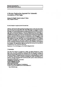
Clear Sky, Tree, Bush Stadium, Stand, People. Leafless Tree, Bush. Street, Building. Football Field, Band. Clear Sky, Sidewalk. Car, People. Track, Banner, Tree.
A Correlation Approach for Automatic Image Annotation⋆ David R. Hardoon1 , Craig Saunders1 , Sandor Szedmak2 , and John Shawe-Taylor1 1
2
University of Southampton, ISIS Research Group, Southampton, U.K. University of Helsinki, Department of Computer Science, Helsinki, Finland
Abstract. The automatic annotation of images presents a particularly complex problem for machine learning researchers. In this work we experiment with semantic models and multi-class learning for the automatic annotation of query images. We represent the images using scale invariant transformation descriptors in order to account for similar objects appearing at slightly different scales and transformations. The resulting descriptors are utilised as visual terms for each image. We first aim to annotate query images by retrieving images that are similar to the query image. This approach uses the analogy that similar images would be annotated similarly as well. We then propose an image annotation method that learns a direct mapping from image descriptors to keywords. We compare the semantic based methods of Latent Semantic Indexing and Kernel Canonical Correlation Analysis (KCCA), as well as using a recently proposed vector label based learning method known as Maximum Margin Robot.
1
Introduction
Due to an increasing rise of multimedia data that is available both on-line and offline, we are faced with the problematic issue of our ability to access or make use of this information, unless the data is organised in such a way that allows efficient browsing, searching and retrieval. One of these issues is image labelling or multilabelling where we would like to annotate an image with several keywords that best describe it. Several solutions have been proposed using keyword association to images and image segments [1, 2, 14, 18]. Recently in [7, 8], it was suggested that methods that use region-based image descriptors generated by automatic segmentation or through fixed shapes may lead to poor performance, as regularly used rectangular regions image descriptors are not robust to a variety of transformations such as rotation. They have suggested using Scale Invariant Feature Transformation (SIFT) [9] feature, which are scale invariant, and utilising them as ‘visual’ terms in a document. We then have a bag-of-visiterms model for each image, and this can then be processed in a similar fashion to bag-of-words models for text documents. ⋆
The authors would like to acknowledge the financial support of the European Community IST Programme; PASCAL Network of Excellence grant no. IST-2002-506778.
In this work we follow the layout suggested by [8] and test their proposed annotation approach with KCCA and Maximum Margin Robot (MMR)[15], a new vector label based learning method. We also suggest learning the association between the keywords and images directly, and therefore learning the association between keywords and particular SIFT descriptors. When a new query image is encountered new keywords could be predicted/genrated according to its SIFT descriptors. The paper is laid-out as follows. In Section 2 we introduce Latent Semantic Indexing and its usage in this context. We continue the semantic model discussion by describing in detail Kernel Canonical Correlation Analysis in Section 3. In Section 4 we discuss Maximum Margin Robot a new vector label based learning method. Section 5 describes the data representation used in this work. This is followed by the experimental setup in Section 6 and our presented results in Section 7. Our final remarks and discussion are given in Section 8.
2
Latent Semantic Indexing
Latent Semantic Indexing (LSI)3 is a classical approach to information retrieval. This approach is a vector based information retrieval method that uses a training collection. Given a term document training matrix A (or image training matrix) with rows as training examples, LSI uses the Singular Value Decomposition (SVD) to factor A into its singular vectors. We are able to apply a noise reduction on the data by projecting the training data into the computed k largest singular vectors. LSI uses this in order to learn the structure of the training collection and to project new test queries into the same semantic space. We are able to write SVD as A′ = U ΣV ′ , where X ′ is the transpose of a matrix or vector X. ˆk V ′ . The rank We denote the k-dimensional approximation of A as A˜′ = Uk Σ k ′ ′ ˜ reduced A is an approximation of the of the original A and Vk is the data in the projected semantic space, which can be seen in the following ˆ −1 )′ . ˆk Vk′ = Σ ˆ −1 Uk′ A˜′ = (AU ˜ kΣ ˆ −1 Uk′ Uk Σ Vk′ = Σ k k k Since we are looking for a similarity measure, we project the query document q into the k semantic feature space of A and D look for theEclosest matching image ˆ −1 will give us the image from the training corpus. Therefore, maxi vik , qUk Σ k from the training corpus with the largest inner project with the query image. Where q is the query image vector and vik are the row vectors of Vk .
3
Kernel Canonical Correlation Analysis
Proposed by Hotelling in 1936, Canonical Correlation Analysis (CCA) is a technique for finding pairs of basis vectors that maximise the correlation between 3
Also known as Latent Semantic Analysis (LSA).
the projections of paired variables onto their corresponding basis vectors. Correlation is dependent on the chosen coordinate system, therefore even if there is a very strong linear relationship between two sets of multidimensional variables this relationship may not be visible as a correlation. CCA seeks a pair of linear transformations one for each of the paired variables such that when the variables are transformed the corresponding coordinates are maximally correlated. Consider the linear combination x = wx′ x and y = wy′ y. Let x and y be two random variables from a multi-normal distribution, with zero mean. The correlation between x and y can be defined as maxwx ,wy ρ = wx′ Cxy wy subject to wx′ Cxx wx = wy′ Cyy wy = 1. Cxx and Cyy are the non-singular within-set covariance matrices and Cxy is the between-sets covariance matrix. We suggest using the kernel variant of CCA [4] since due to the linearity of CCA useful descriptors may not be extracted from the data. This may occur as the correlation could exist in some non linear relationship. The kernelising of CCA offers an alternate solution by first projecting the data into a higher dimensional feature space φ : x = (x1 , . . . , xn ) → φ(x) = (φ1 (x), . . . , φN (x)) (N ≥ n) before performing CCA in the new feature space. Given the kernel functions κa and κb let Ka = XX′ and Kb = YY′ be the kernel matrices corresponding to the two representations of the data. Let X be the matrix whose rows are the vectors φa (xi ), i = 1, . . . , ℓ and similarly Y be a matrix with rows φb (yi ). . Substituting into primal CCA equation gives maxα,β ρ = α′ Ka Kb β subject to α′ K2a α = β ′ K2b β = 1. This is the dual form of the primal CCA optimisation problem given above, which can be cast as a generalised eigenvalue problem and for which the first k generalised eigenvectors can be efficiently found. The theoretical analysis shown in [5] suggests to regularise kernel CCA as it shows that the quality of the generalisation of the associated pattern function is controlled by the sum of the squares of the weight vectors norms. Due to space limitation we refer the reader to [5, 6] for a detailed analysis and the regularised form of KCCA. One aspect we will mention here though is that it is not the case that when using a linear kernel KCCA reduces to standard CCA (see the aforementioned articles for details). Using a linear kernel and KCCA has advantages over CCA, the most prominant of which in our case is speed; this is why we use this variant here. We are able to apply a similar procedure to that used in LSI to find the most matching image from the training corpus to the query image. Whereas here we project the data into the semantic space using a selection of the found eigenvectors corresponding to the largest correlation values. 3.1
Keywords Reconstruction
We are faced with the problem of creating a new document d∗ (i.e. a set of keywords) that best matches our image query. Based on the idea of CCA we are looking for a vector that has maximum covariance to the query image with respect to the weight matrices α and β. Let f = Kxi α, where the vector Kxi contains the kernelised inner products between the query image i and the images
� occurring in the training set. We have maxd∗ f, Wy′ d∗ , where Wy is the matrix containing the weight vectors as rows. The need to use the weight vectors for the documents limits us to the use of linear kernels. For simplicity we assume that the expected structure of the document is of a single keyword that is the most relevant keyword for the query image. Let n be the number of known keywords in the training dataset. We may say that the vector d∗ gives a convex combination of the columns of the identity matrix (i.e. kd∗ k = 1), thus it satisfies the constraints n X
d∗i = 1, d∗i ≥ 0 i = 1, . . . , n.
(1)
i=1
The problem becomes maxd∗ f ′ Wy′ d∗ under the same constraints. Let c = f ′ Wy′ we have maxd∗ cd∗ . Due to the constraints in equation (1) the components of the optimum solution d∗ is equal to � 1 i = arg maxj cj , ∗ (d)i = 0 otherwise. This generates a document containing a single keyword. We modify the original maximisation problem to relax the optimum solution to include keywords above a threshold T . The new relaxed formulation will generate a document with varying number of keywords, depending on T . We are able to use the value of cj to rank the relevance of the selected keywords. We do this by sorting the values of c and taking the keywords relating to the largest values of c above threshold T .
4
Maximum Margin Robot
The Support Vector Machine(SVM) has been shown to be a very useful method of machine learning, but is restricted to directly solving binary classification problems only. There is a strong demand for extending the underlying idea towards multi-class classification and learning when the outputs have complex structure. The known approaches are tackling with the exploding computational complexity and the range of potential applications becomes very limited. There is a straightforward algebraic generalisation of the SVM which can handle arbitrary vector outputs and preserves the same computational complexity of its binary ancestor. The structural learning problems can then be solved via an embedding into a properly chosen vector space. The learning strategy in the vector label learning can be stated as a three-phase process: Embedding: where the structures of the input and output objects are represented in properly chosen Hilbert spaces, reflecting the similarity and the dissimilarity of the objects. Optimisation: has to find the similarity based matching between the input and the output representations, Inversion (Pre-image problem): has to recover the best fitting output structure of its vector representation.
The variant of vector valued learning we introduce was born as a reinterpretation of the variables and parameters occuring in the Support Vector Machine: In the original representation yi ∈ {−1, +1} are binary outputs and w is the normal vector of the separating hyperplane. While in the new representation yi ∈ Y are arbitrary outputs ψ(yi ) ∈ Hψ embedded labels in a linear vector space, and wT is a linear operator projecting the input space into the output space. The output space is a one dimensional subspace in the SVM. The details of reinterpretation of MMR4 are given in Table 1. Due to limited space we refer the reader to [15] where the method is first introduced. Table 1. SVM and MMR interpretation
Binary class learning Vector label learning Support Vector Machine (SVM) Maximum Margin Robot (MMR) min
1 2
wT w +C1T ξ | {z } kwk2 2
w.r.t. w : Hφ → R , normal vec. b ∈ R , bias ξ ∈ Rm , error vector s.t.
yi (wT φ(xi ) + b) ≥ 1 − ξi ξ ≥ 0, i = 1, . . . , m
5
1 2
tr(WT W) +C1T ξ | {z } kWk2 F robenius
W : Hφ → Hψ , linear operator
(2)
b ∈ Hψ , translation(bias) ξ ∈ Rm , error vector D
E ψ(yi ), Wφ(xi ) + b
Hψ
≥ 1 − ξi
ξ ≥ 0, i = 1, . . . , m
Data Representation
There is a great deal of importance on the textural and image means of representation, as we would like to be able to extract as much detailed information as possible for the learning process. Various approaches have been suggested such as colour moments and Gabor texture descriptors[17] as well as scale invariant interest points[10] and affine invariant interest point detector [11]. Scale Invariant Feature Transformation (SIFT) have been introduced by [9] and have been shown to be superior to other descriptors[12]. This is due to the fact that the SIFT descriptors are designed to be invariant to small shifts in position of the salient (i.e. prominent) region. SIFT transforms the image data into scale invariant coordinates relative to local features. The underlying idea of SIFT is 4
MMR code - http://www.ecs.soton.ac.uk/∼ss03v/mmr.html
to extract distinctive invariant features from an image such that it could be used to perform reliable matching between different views of an object or scene. Since we are aiming to learn the association of a keyword to an object, which could appear in different angels and scenes, we find SIFT ideal for the image representation. Documents are usually represented by word frequency. That is, the number of occurrences of each word in the document is counted and a vector of wordfrequencies is created. Although this simplistic approach is usually sufficient for good performance we describe Term Frequency Inverse Document Frequency (TFIDF)[16], which computes the following � � TFIDF(di , wj ) = |{wj ∈ di }| log ℓ |{di ∈ D: wj ∋ di }|−1 . The TFIDF is a means of amplifying the influence of words that occur often in a document but relatively rarely in the whole collection. We apply the TFIDF on the image SIFT descriptors as they were post processed as to mimic the concept of words (SIFT descriptors) in documents (images), the pseudo-details of this procedure are given in the following section and further information can be found in [7]. In the experiments results section we compare the application of TFIDF on the visual terms as well as keeping them as frequency vectors.
6
Experimental Setup
We have used the University of Washington Ground Truth Image Database5 , which contain 697 public-domain images that have been annotated with an average of ∼ 5 keywords per image and with an overall of 287 keywords in the dictionary. [8] has kindly provided us with the post processed data. SIFT descriptors were computed from the images and then clustered using the batch k-means clustering algorithm with random starting points in order to build a vocabulary of ‘visual’ words [7]. Each image in the entire data-set then had its feature vectors quantised by assigning the feature vector to the closest cluster. This amounted into a uniform feature vector of 3000 visual terms. TFIDF was applied on the new image feature vector to amplify the influence of SIFT descriptors that occur often in an image but rarely in the whole set of images. The keywords have been stemmed, having errors corrected and merging plural terms into singular forms. Henceforth the original 287 terms were reduced to 170. We find the frequency of the keywords in the dictionary to be very uneven6 , therefore further reduce the keywords by removing the all keywords that only have one occurrence throughout the database. This rendered us with 132 keywords in the dictionary. The keywords were represent as a frequency vector. We have repeated all experiments 10 times where in each repeat the database was randomly and evenly split into a training and testing set. The 10 repeats 5 6
http://www.cs.washington.edu/research/imagedatabase/ groundtruth/ ∼ 33% of the words have more then 10 occurrences and ∼ 3% have more then 100 occurrences in the database.
are in order to obtain some statistical verification for the used methods. In each run we use the same random split across all methods. We use the same number of dimensional selection k for the LSI semantic project as in [8] (k = 40) since we initially try to reproduce their LSI results. Using the described method in [6, 5] for the selection of the KCCA regularisation parameter we find a regularisation value of τ = 0.2, and by manual testing a feature selection set to 10 to give good results. While the SVD is only applied on the training and query images, KCCA aims to learn the correlation between the training images and their associated keywords. MMR is similar to KCCA but learns the keywords as a multi-label of the images. We use linear kernels across the methods. 6.1
Performance Measure
In order to asses the performance of the discussed methods, we present two complementing measures from the content based retrieval literature. We first consider the normalised score measure, as suggested by [1]. This measure gives a value of 1 if the image is annotated exactly correctly, 0 for predicting nothing or everything and a value of −1 if the exact complement of the original word set is predicted. Throughout the experimentation we multiply this measure by 100. Let r be the number of correctly predicted keywords, n be the number of original keywords, w be the number of incorrectly predicted keywords and N the number of words in the dictionary. We are able to define the normalised score measure to be EN S = r(n)−1 − w(N − n)−1 . The problem with the normalised score measure is that if we consider an annotation method that annotates an image exactly, then the normalised score does not sufficiently weight the incorrect guesses. This was demonstrated by [13], where they have shown that the normalised score is maximised when their annotation system returned 40 keywords per image on a test database with an average of 18.5 keywords per image. This shows that the normalised score may not account for the added noise (i.e. incorrect keywords) once all correct keywords have been selected. We therefore choose to use the precision and recall evaluation as the main measure of the methods performances. We are able define recall as Recall = r(n)−1 , and percision as Precision = r(r + w)−1 . We would like to have a high ratio of correctly annotated keywords to the number of keywords annotated and a high overall ratio of correct keywords (i.e. high precision and high recall).
7
Results
In the following section we present out obtained results. Throughout the presented results, best resutls are highlighted in bold. Initially We present the methods run-time in seconds; KCCA - 2.61, MMR - 0.19 and LSI - 57.42. We find that the vector-label learning algorithm MMR is able to solve the multi-label optimisation problem ∼ 13.74 times faster than KCCA and ∼ 302.2 times faster than applying the SVD procedure.
In our first task we aim to annotate a query by retrieving to it the most similar image from the training corpus. The query image is then annotated with the keywords from the found matching image. In this task we compare KCCA, MMR and LSI, we also provide an indication of how good the image annotation approach would perform if the “matching” image would have been drawn randomly from the training corpus. In Tables 2 and 3 we give the normalised score measure for the methods on the testing and training set.
Table 2. Image Retrieval Results Comparison (Train Set) Method KCCA (10) - TFIDF MMR - TFIDF LSI (40) - TFIDF KCCA (10) - FV MMR - FV LSI (40) - FV
Precision 68.77% ± 1.38% 36.98% ± 5.43% 20.34% ± 5.04% 68.45% ± 1.56% 31.28% ± 1.95% 20.67% ± 2.81%
Recall 80.79% ± 1.29% 35.99% ± 2.41% 21.07% ± 5.67% 80.42% ± 1.60% 24.08% ± 2.24% 20.64% ± 2.98%
ENS 79.41 ± 1.34 33.07 ± 2.50 17.42 ± 5.15 79.03 ± 1.67 28.47 ± 2.01 17.67 ± 2.96
We are able to observe that all methods are able to find on average matching images that contain keywords that do not contain everything or nothing (an EN S value of 0), but that KCCA with a feature selection of 10 is able to find more images with a similar keyword annotation. It is surprising to observe that LSI and Random have a similar performance level. As discussed in the previous section the normalised score measure may not be an ideal performance measure, therefore we provide in Table 2 the precision and recall performance on the training set and in Table 3 the precision and recall performance measure on the testing set. We again observe that LSI on average has a similar performance to random. Although as indicated by the large standard deviation, there are random splits of training and testing that produce a recall and precision value of ∼ 35%. We are assured that learning is occurring when we compare KCCA and
Table 3. Image Retrieval Results Comparison (Test Set) Method KCCA (10) - TFIDF MMR - TFIDF LSI (40) - TFIDF KCCA (10) - FV MMR - FV LSI (40) - FV Random
Precision 37.01% ± 1.22% 34.15% ± 5.32% 19.97% ± 5.44% 36.58% ± 1.37% 21.73% ± 1.44% 19.31% ± 3.23% 19.27% ± 0.92%
Recall 45.92% ± 1.11% 32.95% ± 1.39% 20.54% ± 5.82% 45.14% ± 1.46% 29.11% ± 1.48% 18.93% ± 2.82% 19.21% ± 0.92%
ENS 42.95 ± 1.16 29.96 ± 1.44 17.08 ± 5.58 42.23 ± 1.46 26.30 ± 1.44 16.30 ± 3.36 16.26 ± 0.9
MMR to random. We are able to see that MMR produces twice the recall and precision and KCCA twice the performance of precision and ∼ 2.5 times of recall. We find that the application of TFIDF on the ‘visual’ terms does boost results implying that increasing the weighting of SIFT descriptors that occur frequently within an image but not so in overall images, helps the learning process. We were unable to reproduce the LSI results given in [8] where it performed best. In Table 4 we give an example of three query images and the keywords of the retrieved images from the various methods. We do not display the actual retrieved images due to lack of space. Table 4. Image Annotation via Matching Image Retrieval
Original
MMR
KCCA
LSI
Tree Trunk, Log Ground, Elk Greenery Building, Tree, Grass Leafless Tree, Bush Clear Sky, Sidewalk
Partially Cloudy Sky Tree, Water Hill Clear Sky, Tree, Bush Street, Building Car, People
Tree Trunk, Log Ground, Elk Greenery Ocean, Building Tree, Sky
Partially Cloudy Sky Ground, Water, Hill Tree, Grass Sky, Cloud, Building Ocean
Football Field, Band Partially Cloudy Sky Track, Tree, Post Stadium, Stand, People Football Field, Band Track, Banner, Tree Post Cloudy Sky, Bridge Water Cloud, Tree, Palace
In the second experiment we aim to predict a multi-label using the MMR and generate a new best matching document to the query using KCCA. In both methods we predict/create a new document containing the exact number of keywords as with the original query. In Tables 5 and 6 we again provide the normalised score measure for completeness. We are able to observe that here the performance of random extremely degrades from that quoted performance in Tables 2 and 3 while that of KCCA and MMR stays similar. In Table 5 we give the performance on the training set and in Table 6 the performance on the testing set is displayed. We notice that the recall and precision values are equivalent to each other, we presume that this occurs due to the fact that for each query image we predict/create a different set of keywords (according to the number of keywords in the query image).
We observe that although we are now trying to predict/generate keywords directly from an image rather than finding a similar image and using its keywords, our results are similar across the two approaches. This similarity is not surprising as in both approaches we are learning the association between images and words and not images to images, we only change our testing criterion in each annotation procedure. We find as in the previous annotation approach that the application of TFIDF increases the methods performance. Table 5. Keyword Generation Results Comparison (Train Set) Method KCCA (10) - TFIDF MMR -TFIDF KCCA (10) - FV MMR - FV
Precision & Recall 68.1% ± 1.28% 37.12% ± 0.96% 68.50% ± 1.36% 28.30% ± 1.43%
ENS 67.01 ± 1.29 34.78 ± 1.01 67.42 ± 1.38 25.64 ± 1.49
Table 6. Keyword Generation Results Comparison (Test Set) Method KCCA (10) MMR KCCA (10) - FV MMR - FV Random
Precision & Recall 38.16% ± 1.41% 31.42% ± 1.77% 36.80% ± 1.36% 23.75% ± 2.05% 3.63% ± 0.37%
ENS 36.06 ± 1.43 28.9 ± 1.82 34.60 ± 1.38 20.97 ± 2.09 0.13 ± 0.28
In Table 7 we give an example of three query images and the keywords that were predicted/generated from the various methods. While performing quite accurately on image 1 it is interesting to observe that in image 2 MMR replaced Cloud with Snow, while KCCA learnt the association of the keywords which described the surroundings of the image. The third image query shows a more complicated example due to the density of elements within it. It is visible that MMR keyword prediction, except for Fields, could not really describe the image although Water Fall and Duck Pond could be somewhat understood as there is water in the image. KCCA generated an incorrect annotation of Building probably due to the high density of trees which could resemble the structure of a building. We find that in both image annotation procedures KCCA and MMR perform extremely well in comparison to LSI and random, indicating that 1) learning the association of keywords to image descriptors using superior semantic models can produce good results and 2) we are able to learn the association as a multi-label
Table 7. Keyword Generation
Original Tree, Clear Sky, People Stands, Football Field Scoreboard, Stadium MMR Stadium, Football Field Cloudy Sky, People Track, Band, Tree KCCA Tree, Pole, Struct People, Overcast Sky Football Field,Car
Tree, Sky, Cloud Temple
Tree Trunk, Water Greenery, Elk
Snow, Sky, Temple, Tree
Water Fall, Fields, Red Square Duck Pond Ground, Grass, Tree Building
Overcast Sky,, Tree Partially Cloudy Sky Ground
task while retaining the complexity of the learning to a practical minimum. It is interesting in to note that while applying TFIDF on the visual terms boosts results for both LSI and MMR, KCCA seems to stay constant in its keyword prediction and annotation performance. We believe that this shows that even without increasing the weighting of frequently occurring SIFT descriptors within an image, KCCA is able to find matching correlation between the keywords and those SIFT descriptors.
8
Conclusions
Two annotation procedures were presented; the first aiming to retrieve an image best matching a query image and the second aiming to annotate a query image directly. We have shown that the direct annotation can produce as good results as an image comparison. Although the analogy of annotating an image based on the most similar image is adequate we believe that learning the relationship between keywords and image descriptors to be a more interesting and challenging task. In our results we show that it is indeed possible to learn this association directly and still provide good results. In future work we would like to explore enhancing the annotation accuracy by combining several image descriptors[3] as well as examining a new non orthogonal representation of the keywords as labels for the MMR method. Further work on KCCA parameter selection and experimental reproduction on a larger database.
References 1. Kobus Barnard, Pinar Duygulu, David Forsyth, Nando de Fretias, David M. Blei, and Michael I. Jordan. Matching words and pictures. Journal of Machine Learning Research, 3:1107–1135, 2003. 2. D. Blei and M. Jordan. Modeling annotated data. In Proc. of the 26th Intl. Association for Computing Machinery Special Interest Group Information Retrieval Conference (ACM SIGIR), 2003. 3. Jason D. R. Farquhar, David R. Hardoon, Hongying Meng, John Shawe-Taylor, and Sandor Szedmak. Two view learning: SVM-2K, theory and practice. In Advances of Neural Information Processing Systems 19, 2005. 4. Colin Fyfe and Pei Ling Lai. Kernel and nonlinear canonical correlation analysis. International Journal of Neural Systems, 2001. 5. David R. Hardoon. Semantic Models for Machine Learning. PhD thesis, University of Southampton, 2006. 6. David R. Hardoon, Sandor Szedmak, and John Shawe-Taylor. Canonical correlation analysis: an overview with application to learning methods. Neural Computation, 16:2639–2664, 2004. 7. Jonathon S. Hare and Paul H. Lewis. On image retrieval using salient regions with vector spaces and latent semantics. In Image and Video Retrieval: Third International Conference (CIVR), 2005. 8. Jonathon S. Hare and Paul H. Lewis. Saliency-based models of image content and their application to auto-annotation by semantic propagation. In Proceedings of Multimedia and the Semantic Web / European Semantic Web Conference, 2005. 9. D.G. Lowe. Object recognition from local scale-invariant features. In Proceedings of the 7th IEEE International Conference on Computer vision, pages 1150–1157, Kerkyra Greece, 1999. 10. K. Mikolajczyk and C. Schmid. Indexing based on scale invariant interest points. In Proceedings of the 2001 IEEE Computer Society Conference on Computer Vision and Pattern Recognition, pages 525–531, Hawaii USA, 2001. 11. K. Mikolajczyk and C. Schmid. An affine invariant interest point detector. In Proceedings of the 2002 European Conference on Computer vision, pages 128–142, Copenhagen Denmark, 2002. 12. K. Mikolajczyk and C. Schmid. Indexing based on scale invariant interest points. In International Conference on Computer Vision and Pattern Recognition, pages 257–263, 2003. 13. F. Monay and D. Gatica-Perez. On image auto-annotation with latent space models. In MULTIMEDIA ’03: Proceedings of the eleventh ACM international conference on Multimedia. ACM Press, 2003. 14. J.-Y. Pan, H.-J. Yang, C. Faloutsos, and P. Duygulu. Gcap: Graph-based automatic image captioning. In Proc. of the 4th International Workshop on Multimedia Data and Document Engineering (MDDE 04), in conjunction with Computer Vision Pattern Recognition Conference (CVPR 04), 2004. 15. J. Rousu, C.J. Saunders, S. Szedmak, and J. Shawe-Taylor. Learning hierarchical multi-category text classification models. In ICML. 2005. 16. G. Salton and M. J. McGill. Introduction to Modern Information Retrieval. McGraw-Hill, Berlin, 1983. 17. N. Sebe, Q. Tian, E. Loupias, M. Lew, and T. Huang. Evaluation of salient point techniques. Image and Vision Computing, 21:1087–1095, 2003. 18. E. P. Xing, R. Yan, and A. G. Hauptmann. Mining associated text and images using dual-wing harmoniums. In Uncertainty in Artificial Intelligence ’05, 2005.