arXiv:math/0611573v1 [math.NA] 19 Nov 2006
A counterexample concerning the L2-projector onto linear spline spaces Peter Oswald International University Bremen e-mail:
[email protected]
Abstract For the L2 -orthogonal projection PV onto spaces of linear splines over simplicial partitions in polyhedral domains in IRd , d > 1, we show that in contrast to the one-dimensional case, where kPV kL∞ →L∞ ≤ 3 independently of the nature of the partition, in higher dimensions the L∞ -norm of PV cannot be bounded uniformly with respect to the partition. This fact is folklore among specialists in finite element methods and approximation theory but seemingly has never been formally proved.
1
Introduction
Variational methods based on piecewise polynomial approximations are a workhorse in numerical methods for PDEs and data analysis. In particular, least-squares methods lead to the study of the L2 -orthogonal projection operator PV : L2 (Ω) → V onto a given spline space V defined on a domain Ω ∈ IRd . A question of considerable interest is the uniform boundedness of the L∞ -norm kPV kL∞ →L∞ :=
max
f ∈L∞ (Ω): kf kL∞ =1
kPV f kL∞
of PV with respect to families of spline spaces V . If Ω is a bounded interval in IR1 , then the question has been intensively studied for the family of spaces of smooth splines of fixed degree r over arbitrary partitions, where Shadrin [7] has recently established that kPV kL∞ →L∞ ≤ C(r) < ∞,
r ≥ 1,
(1)
for any partition. This result was known for a long time for small values of r, e.g., Ciesielski [3] proved that for linear splines one can take C(1) = 3, while de Boor [2] solved the case r ≤ 4. The estimate (1) plays an important role in numerical analysis and for the investigation of orthonormal spline systems such as the Franklin system in Lp -based scales of function spaces, 1 ≤ p ≤ ∞. 1
In higher dimensions, the study of the L∞ -norm of PV arose mostly in the context of obtaining Lp error estimates in the finite element Galerkin method [5, 6], where sufficient conditions on the underlying partition and nodal basis {φi } of a finite element space V are formulated under which the norms kPV kL∞ →L∞ are bounded by a certain finite constant. Interestingly enough, these results suggest that such conditions on partitions resp. finite element type are essential for obtaining uniform bounds but formal proof of their necessity was not given. Similarly, in the theory of multivariate splines final results on the uniform boundedness of kPV kL∞ →L∞ could not be localized. Recently, Ciesielski [4] asked about the extension of his result for linear splines [3] to the higher-dimensional case, and the unanimous opinion of the audience was that in higher dimensions a similar result cannot hold. However, other than a vague reference to unpublished work by A. A. Privalov, no concrete proof could be found. It is the aim of this note to provide an elementary example of triangulations TJ of a square Ω ⊂ IR2 into O(J) triangles for which kPV (TJ ) kL∞ →L∞ ≥ J,
J ≥ 1,
(2)
where V (TJ ) is the space of linear C 0 splines (or finite element functions) on TJ ; see Theorem 1 below. As J → ∞, the triangulations TJ will not satisfy the minimum angle condition, which is natural since for these types of triangulations a uniform bound can easily be established. However, they satisfy the maximum angle condition, [1], and do not possess vertices of high valence. The example can easily be extended to d ≥ 3, and implies that C(1) = ∞ for all d > 1.
2
Notation and Result
We concentrate on d = 2, the case d ≥ 3 is mentioned in Section 3. Let Ω ⊂ IR2 be a bounded polygonal domain equipped with a finite triangulation T into non-degenerate closed triangles ∆ satisfying the usual regularity condition that two different triangles may intersect at a common vertex resp. edge only. The set of vertices of T is denoted by VT . Let |E| denote the Lebesgue measure of a measurable set E ⊂ IR2 . By 0 < αT ≤ α ¯ T < π we denote the minimal and maximal interior angle of all triangles in T . Let V (T ) denote the linear space of all continuous functions g whose restriction to any of the triangles ∆ ∈ T is a linear polynomial. Any g ∈ V (T ) has a unique representation of the form X g= g(P )φP , (3) P ∈VT
where the Courant hat functions φP ∈ V (T ) are characterized by the conditions φP (P ) = 1, and φP (Q) = 0, where Q 6= P is any of the remaining vertices of T . Thus, dim V (T ) = #VT , and supp φP = ΩP := ∪∆∈T : P ∈∆ ∆. The set ΩP corresponds to the 1-ring neighborhood of P in T , and we denote by VP = {Q ∈ ΩP ∩ V : Q 6= P } the set of all neighboring vertices to P . 2
The L2 -orthogonal projection of a function f ∈ L2 (Ω) onto V (T ) is given by the unique g := PV (T ) f ∈ V (T ) such that (f − g, φP ) = 0
∀ P ∈ VT .
Here and in the sequel, (·, ·) stands for the L2 (Ω) inner product. Using (3) with unknown nodal values xP = g(P ) as ansatz, this is equivalent to the linear system X
(φQ , φP )xQ = (f, φP )
∀ P ∈ V.
(4)
Q∈V
A simple calculation shows that (φP , φP ) =
|ΩP | . 6
Similarly, if Q ∈ VP is a neighbor of P then (φQ , φP ) =
|∆| , ∆∈T : P,Q∈∆ 12 X
in all other cases we have (φQ , φP ) = 0. This shows in particular that (φP , φP ) =
X
(φQ , φP ) = (1, φP )/2.
Q6=P
I.e., if we normalize in (4) by (φP , φP ) then (4) turns into a linear system Ax = b,
x := (xQ : Q ∈ VT )T ,
b := (bP =
(f, φP ) : P ∈ VT )T , (φP , φP )
(5)
where kbk∞ ≤ 2kf kL∞ , and A := (aP Q ) satisfies
and
aP Q =
1=
X
Q6=P
1, (φQ ,φP ) (φP ,φP )
0,
aP Q =
X
Q = P, > 0, Q ∈ VP , otherwise, aP Q ,
(6)
∀ P ∈ VT .
(7)
Q∈VP
Thus, the matrix A is only weakly diagonally dominant, and not strictly diagonally dominant as in the one-dimensional case. Otherwise, we could estimate kA−1 k∞ in a trivial way, and use the inequality kPV (T ) kL∞ →L∞ ≤ 2kA−1 k∞ = 2 max
kAyk∞ ≤1
kyk∞,
(8)
which follows from the above, in conjunction with the obvious equality kPV (T ) f kL∞ = kxk∞ . Let us mention without proof that (8) implies the following partial result. 3
Proposition 1 If for any two neighboring vertices P 6= Q from VT we have aP Q ≥ c0 > 0, then kPV (T ) kL∞ →L∞ ≤ (1 + 2c0 )c−2 0 . For triangulations satisfying the minimum angle condition uniformly, i.e., αT ≥ α0 > 0, this result is applicable with a c0 determined solely by α0 , and thus covers the bounds considered in the finite element literature [5, 6]. The main result of this note is the following Theorem 1 For any J ≥ 1, there is a triangulation TJ of a square into 8J + 4 triangles such that the norm of the L2 -projector PV (TJ ) satisfies kPV (TJ ) kL∞ →L∞ ≥ 2J. Thus, for spatial dimension d = 2 we have C(1) := sup kPV (T ) kL∞ →L∞ = ∞. T
We conjecture that in terms of the number of triangles our result is asymptotically sharp for bounded polygonal domains in IR2 , i.e., sup T : #T ≤N
kPV (T ) kL∞ →L∞ ≍ N,
N → ∞.
(9)
That Ω is a square is not crucial. The examples given below can easily be modified to show C(1) = ∞ for simplicial partitions in higher dimensions as well.
3
Proof of Theorem 1
We will use the following notation. Let Sa = [−a, a]2 be the square of side-length 2a, a > 0, with center at the origin. Set Ω := S1 , with vertices denoted (in clockwise direction) by P0,i , i = 1, . . . , 4, and fix the parameter t ∈ (0, 1). The triangulation TJ , J ≥ 1, of Ω is obtained by inserting the squares St , St2 ,. . . , StJ , whose vertices will be denoted similarly by Pj,i, i = 1, . . . , 4, j = 1, . . . , J, placing an additional vertex PJ+1 at the origin, connecting PJ+1 by straight lines with the 4 vertices P0,i of S1 , and finally subdividing each of the remaining trapezoidal regions Pj−1,i−1Pj,i−1Pj,i Pj−1,i into two triangles by connecting Pj−1,i−1 with Pj,i in a consistent way. The outer rings of the resulting triangulation are shown in Fig. 1 a). Let the function f ∈ L∞ (Ω) with kf kL∞ = 1 be defined as follows: j
f (x) = (−1) ,
x ∈ Ωj :=
(
Stj−1 \Stj , j = 1, . . . , J, StJ , j = J + 1.
We use the same notation as above, and consider the linear system (5) corresponding to the L2 -orthogonal projection g = PV (TJ ) f of this f onto V (TJ ). Because of uniqueness of orthogonal projections and the rotational symmetry of TJ and f , the entries of the vector 4
1
1
P
P
1,1
1,2
0
P
1,3
−1 −1
P
P
1,4
1,4
−1
1
0
1
Figure 1: Triangulation TJ for t = 0.3 (left), and typical ΩPj,i (right) x that represent the nodal values of g corresponding to the vertices Pj,i, i = 1, . . . , 4, are equal, and will be denoted by xj , j = 0, . . . , J (the value at the origin is denoted by xJ+1 ). Moreover, the 4 equations in (5) corresponding to the 4 vertices of a square Stj , j = 0, . . . , J, can be replaced by one, thus turning the original system Ax = b of ˜x = ˜b of dimension J + 2 for the dimension 4J + 5 into a reduced tridiagonal system A˜ T vector x˜ = (x0 , . . . , xJ+1 ) . Since the equations in the system (5) are invariant under affine transformations, and because of the definition of TJ via squares Stj shrinking at a fixed geometric rate, it is easy to see that, with the exception of the first and last two, ˜x = ˜b have the same form: all equations in A˜ αxj−1 + βxj + γxj+1 = (−1)j δ,
j = 1, . . . , J − 1.
(10)
The coefficients can be found from the triangular neighborhood ΩPj,i of any of the Pj,i, j = 1, . . . , J − 1 (see Fig. 1 for an illustration), and the definitions leading to (5). We do not need their exact coefficient expressions, just their limit behavior as t → 0, i.e., we will be looking for the entries of Aˆ := limt→0 A˜ and ˆb := limt→0 ˜b. Indeed, since for t → 0 the whole is essentially covered by the single triangle with vertices Pj,i, Pj−1,i−1, Pj−1,i, and since f (x) = (−1)j on the latter, we have α = 1 + O(t),
β = 1 + O(t),
γ = O(t2 ),
δ = 2 + O(t).
From (10), we obtain in the limit t → 0 the equations xˆj−1 + xˆj = 2(−1)j ,
j = 1, . . . , J − 1,
where xˆj = limt→∞ xj (the existence of these limits follows from the invertibility of the ˆ see below). Similar considerations for the first and the last two equations limit matrix A, 5
˜x = ˜b yield the remaining three equations of Aˆ ˆx = ˆb as follows: of A˜ 1 3 xˆ0 + xˆ1 = −2, 2 2
xˆj−1 + xˆj = 2(−1)j ,
j = J, J + 1.
The resulting matrix Aˆ is obviously invertible. After finding xˆ0 = xˆ1 = −1 from the first two equations, forward substitution gives xˆj = (2j − 1)(−1)j , j = 2, . . . , J + 1. This implies that for any ǫ > 0 one can find a sufficiently small t > 0 such that k˜ xk∞ ≥ kˆ xk∞ − ǫ = 2J + 1 − ǫ. This proves Theorem 1. Note that the above reasoning does not work for type-I triangulations of a square obtained from a non-uniform rectangular tensor-product partition. We conclude with the straightforward extension of the above example to arbitrary d > 2. Let em denote the m-th unit coordinate vector in IRd , m = 1, . . . , d. As Ω we take the convex polyhedral domain with vertices P0,1 = e1 + e2 ,
P0,2 = e1 − e2 ,
P0,3 = −e1 − e2 ,
P0,4 = −e1 + e2 ,
and Pm′ = em , m = 3, . . . , d. For d = 3, this domain is a pyramid with square base in the xy-plane, and tip on the z-axis. A suitable simplicial partition of Ω is obtained as follows. The base square with vertices P0,i , i = 1, . . . , 4, is triangulated into TJ which depends on the parameters 0 < t < 1 and J as described for d = 2. The resulting triangulation (now embedded into IRd ) and its vertices are again denoted by TJ resp. by Pj,i, i = 1, . . . , 4, j = 0, . . . , J, and PJ+1 . Then each simplex in the associated simplicial partition PJ of Ω is generated by the d − 2 vertices Pm′ , m = 3, . . . , d, and the three vertices of a triangle in TJ . The latter is called base triangle of the associated simplex. Obviously, the d-dimensional volume of each simplex is proportional to the 2-dimensional area of its base triangle, with proportionality constant 2/d!. To obtain a suitable function f ∈ L∞ (Ω) with kf kL∞ = 1 we prescribe values ±1 on the simplices by inheritance from the values on the base triangles of the above 2-dimensional f . From the symmetry properties of f and PJ , it is obvious that the L2 -orthogonal projection PV (PJ ) f of f onto the linear spline space V (PJ ) is characterized by its value xJ+1 at the origin PJ+1 , by values xj taken at the vertices Pj,i, i = 1, . . . , 4, where j = 0, . . . , J, and a common value x′ taken at the remaining vertices Pm′ , m = 3, . . . , d. To estimate these values which, in complete analogy to the 2-dimensional case, are ˜x = ˜b (now of dimension represented by the solution vector x˜ of a certain linear system A˜ ˆx = ˆb of this linear system for t → 0. We spare the J + 3), we need the limit version Aˆ reader the elementary calculations, and state it without proof: d−2 ′ d+2 xˆ = (−1)j , 2 2 3 1 d−2 ′ d+2 xˆ0 + xˆ1 + xˆ = − , 2 2 2 2 d−3 ′ d+2 1 )ˆ x = − . xˆ0 + xˆ1 + (1 + 2 2 2 xˆj + xˆj−1 +
6
j = 1, . . . , J + 1,
From this system one easily concludes that kˆ xk∞ ≥ cJ, and consequently kPV (PJ ) f kL∞ ≥ cJ for a small enough t > 0 which implies the desired result. The lower bound cJ obtained does not seem to accurately reflect the possible growth of the projector norms in L∞ as a function of the number of simplices, for d ≥ 3 we would rather expect an exponential rate.
References [1] I. Babuska, A. K. Aziz, On the angle condition in the finite element method, SIAM J. Numer. Anal. 13 (1976), 214–226. [2] C. de Boor, On a max-norm bound for the least-squares spline approximant, in Approximation and Function Spaces (Gdansk, 1979), Z. Ciesielski (ed.), pp. 163– 175, North-Holland, Amsterdam, 1981. [3] Z. Ciesielski, Properties of the orthonormal Franklin system, Studia Math. 23 (1963), 141–157. [4] Z. Ciesielski, Private communication, Int. Conf. Approximation Theory and Probability, Bedlowo, 2004. [5] J. Desloux, On finite element matrices, SIAM J. Numer. Anal. 9, 2 (1972), 260–265. [6] J. Douglas, Jr., T. Dupont, L. Wahlbin, The stability in Lq of the L2 -projection into finite element function spaces, Numer. Math. 23 (1975), 193–197. [7] A. Yu. Shadrin, The L∞ -norm of the L2 -spline projector is bounded independently of the knot sequence: a proof of de Boor’s conjecture, Acta Math. 187 (2001), 59–137.
7