Electronic Research Archive of Blekinge Institute of Technology http://www.bth.se/fou/ This is an author produced version of a conference paper. The paper has been peer-reviewed but may not include the final publisher proof-corrections or pagination of the proceedings.
Citation for the published Conference paper: Title: A CUDA Implementation of Random Forests - Early Results Author: Håkan Grahn, Niklas Lavesson, Mikael Hellborg Lapajne, Daniel Slat
Conference Name: Third Swedish Workshop on Multi-core Computing
Conference Year: 2010 Conference Location: Göteborg Access to the published version may require subscription. Published with permission from: Chalmers Institute of Technology
A CUDA Implementation of Random Forests - Early Results Håkan Grahn, Niklas Lavesson, Mikael Hellborg Lapajne, and Daniel Slat School of Computing, Blekinge Institute of Technology SE-371 79 Karlskrona, Sweden
[email protected],
[email protected]
ABSTRACT Machine learning algorithms are frequently applied in data mining applications. Many of the tasks in this domain concern high-dimensional data. Consequently, these tasks are often complex and computationally expensive. This paper presents a GPU-based parallel implementation of the Random Forests algorithm. In contrast to previous work, the proposed algorithm is based on the compute unified device architecture (CUDA). An experimental comparison between the CUDA-based algorithm (CudaRF), and state-of-the-art parallel (FastRF) and sequential (LibRF) Random forests algorithms shows that CudaRF outperforms both FastRF and LibRF for the studied classification task.
1.
INTRODUCTION
Machine learning (ML) algorithms are frequently applied in data mining and knowledge discovery. The process of identifying patterns in high-dimensional data is often complex and computationally expensive, which result in a demand for high performance computing platforms. Random Forests (RF) [1] has been proven to be a competitive algorithm regarding both computation time and classification performance. Further, the RF algorithm is a suitable candidate for parallelization. This has already been exploited, e.g., the Fast Random Forests (FastRF) algorithm in the Weka machine learning workbench [13]. Graphics processors (GPUs) are today extensively employed for non-graphics applications, and the area is often referred to as General-purpose computing on graphics processing units, GPGPU [3, 4]. Initially, GPGPU programming was carried out using shader languages such as HLSL, GLSL, or Cg. However, there was no easy way to get closer control over the program execution on the GPU. The compute unified device architecture (CUDA) is an application programming interface (API) extension to the C programming language, and contains a specific instruction set architecture for access to the parallel compute engine in the GPU. Using CUDA, it is possible to write (C-like) code for the GPU, where selected
segments of a program are executed on the GPU while other segments are executed on the CPU. Several machine learning algorithms have been successfully implemented on GPUs, e.g., neural networks [10], support vector machines [2], and the Spectral clustering algorithm [11]. However, it has also been noted on multiple occasions that decision tree-based algorithms may be difficult to optimize for GPU-based execution. To our knowledge, GPU-based Random Forests have only been investigated in one previous study [9], where the RF implementation was done using Direct3D and the high level shader language (HLSL). In this paper, we present a highly parallel CUDA-based implementation of the Random Forests algorithm. The algorithm is experimentally evaluated on a NVIDIA GT220 graphics card with 48 CUDA cores and 1 GB of memory. The performance is compared with two state-of-the-art implementations of Random Forests; one sequential, i.e., LibRF [6], and one parallel, i.e., FastRF in Weka [13]. Our results show that the CUDA implementation is 2.9 − 4.2 times faster than FastRF and 7.7 − 9.2 times faster than LibRF for 128 trees and k-values between 6 and 16. The rest of the paper is organized as follows. Section 2 presents the random forests algorithm, and Section 3 presents CUDA and the GPU architecture. Our CUDA implementation of Random Forests is described in Section 4. The experimental methology and the results are presented in Section 5 and Section 6, respectively. Finally, we discuss and conclude our findings in Section 7.
2.
RANDOM FORESTS
The concept of Random Forests (RF) was first introduced by Leo Breiman [1]. It is an ensemble classifier consisting of decision trees. The idea behind Random Forests is to build many decision trees from the same data set using bootstrapping and randomly sampled variables to create trees with variation. The bootstrapping generates new data sets for each tree by sampling examples from the training data uniformly and with replacement. These bootstraps are then used for constructing the trees which are then combined in to a forest. This has proven to be effective for large data sets with missing attributes values [1]. Each tree is constructed by the principle of divide-and-conquer. Starting at the root node the problem is recursively broken down into sub-problems. The training instances are thus
divided into subsets based on their attribute values. To decide which attribute is the best to split upon in a node, k attributes are sampled randomly for investigation. The attribute that is considered as the best among these candidates is chosen as split attribute. The benefit of splitting on a certain attribute is decided by the information gain, which represents how good an attribute can separate the training instances according to their target attribute. As long as splitting gives a positive information gain, the process is repeated. If a node is not split it becomes a leaf node, and is given the class attribute that is the most common occurring among the instances that fall under this node. Each tree is grown to the largest extent possible, and there is no pruning.
Thread synchronization through the shared memory is only supported between threads running on the same SM. The GPU is then built by combining a number of SMs. The graphics card also contains a number of additional memories that are accessible from all SPs, i.e., the global (often refer to as the graphics memory), the texture, and constant memories. Multiprocessor N Multiprocessor 2
Shared memory
When performing classifications, the input query instances traverse each tree which then casts its vote for a class and the RF considers the class with the most votes as the answer to a classification query. There are two main parameters that can be adjusted when training the RF algorithm. First, the number of trees can be set by the user, and second, there is the k value, i.e., the number of attributes to consider in each split. These parameters can be tuned to optimize classification performance for the problem at hand. The random forest error rate depends on two things [1]: • The correlation between any two trees in the forest. Increasing the correlation increases the forest error rate. • The strength of each individual tree in the forest. A tree with a low error rate is a strong classifier. Increasing the strength of the individual trees decreases the forest error rate. Reducing k reduces both the correlation and the strength. Increasing it increases both. Somewhere in between is an optimal range of k. By watching the classification accuracy for different settings a good value of k can be found. Creating a large number of decision trees sequentially is ineffective when they are built independently of each other. This is also true for the classification (voting) part where each tree votes sequentially. Since the trees in the forest are independently built both the training and the voting part of the RF algorithm can be implemented for parallel execution. An RF implementation working in this way would have potential for great performance gains when the number of trees in the forest is large. Of course the same goes the other way; if the number of trees in the forest is small it may be an ineffective approach. This will become clearer when looking at our architecture and implementation in Section 4 of the document.
3.
CUDA AND GPU ARCHITECTURE
The general architecture for the NVIDIA GPUs that supports CUDA is shown at the top of Fig. 1. The GPU has a number of CUDA cores, a.k.a. shader processors (SP). Each SP has a large number of registers and a private local memory (LM). Eight SPs together form a streaming multiprocessor (SM). Each SM also contains a specific memory region that is shared among the SPs within the same SM.
Shared memory
Multiprocessor 1 Shared memory SP
SP SP
SP
SP LM
LM
LM
SP
LM
SP
SP
SP LM
LM
LM
LM
LM
Global Memory
Property CUDA cores Compute capability Graphics/Processor clock Total amount of memory Memory interface
Value 48 1.2 625 MHz/1.36 GHz 1 GB 128-bit DDR3, 25.3 GB/s
Figure 1: The GPU architecture assumed by CUDA (upper), and the main characteristics for the NVIDIA GeForce GT220 graphics card (lower). The GPU used for algorithm development and experimental evaluation in the presented study is the Nvidia GT220. The relevant characteristics of this particular GPU is described at the bottom of Fig. 1. In order to utilize the GPU for computation, we must transfer all data from the host memory to the GPU memory, thus the bus bandwidth and latency between the CPU and the GPU may become a bottleneck. A CUDA program consists of two types of code: sequential code executed on the host CPU and CUDA functions, or ’Kernels’, launched from the host and executed in parallel on the GPU. Before a kernel is launched, the required data (e.g., arrays) must have been transferred from the host memory to the device memory, which can be a bottleneck [8]. When data is placed in the GPU, the CUDA kernel is launched in a similar way as calling a regular C function. When executing a kernel, a number of CUDA threads are created and each thread executes an instance of that kernel. Threads are organized into blocks with up to three dimensions, and then, blocks are organized into grids, also with up to three dimensions. The maximum number of threads per block and number of blocks per grid are hardware dependent. In the CUDA programming model, each thread is assigned a local memory that is only accessible by the thread. Each block is assigned a shared memory for com-
munication between threads in that block, while the global memory which is accessible by all threads executing the kernel. The CUDA thread hierarchy is directly mapped to the hardware model of GPUs. A device (GPU) executes kernels (grids) and each SM executes blocks. To utilize the full potential of a CUDA-enabled NVIDIA GPU, thousands of threads should be running, which requires a different program design than for today’s multi-core CPUs.
4. A CUDA IMPLEMENTATION OF RF 4.1 Basic assumptions and execution flow Both the training phase and the classification phase are parallelized in our CUDA implementation. The approach taken is similar to the one in the study by Topic et al. [12]. In our implementation we use one CUDA thread to build one tree in the forest, since we did not find any straight-forward approach to build individual trees in parallel. Therefore, our implementation works best for a large number of trees. Many decision tree algorithms are based on recursion, e.g., both the sequential and parallel Weka algorithms are based on recursion. However, the use of recursion is not possible in the CUDA-based RF algorithm since there is no support for recursion in kernels executed on the graphics device. Therefore, it was necessary to design an iterative tree generator algorithm. The following steps illustrate the main execution steps in our implementation. Further, Figure 2 shows which parts of the execution that are done on the host CPU and on the device GPU, respectively, as well as the data transfers that take place between the host and the device (GPU). Steps 2-8 are repeated N times when N -fold cross-validation is done.
Figure 2: Execution flow and communication between Host and Device for CudaRF. 7. The execution returns to the host and the results are transferred from the device memory to the host memory. 8. The results are presented on the host.
1. Training and query data is read from an ARFF data set file to the host memory. 2. The training data is formatted and missing attribute values are filled in, and then the data is transferred to the device memory. 3. (a) A CUDA kernel with one thread per tree in the forest is launched. A parallel kernel for the bagging process is executed where each tree gets a list of which instances to use. Instances not used by a tree are considered as the out of bag (oob) instances for that tree. (b) The forest is constructed in parallel on the GPU using as many threads as there shall be trees in the forest. (c) When the forest is completely built, each tree performs a classification run on its oob instances. The results of the oob run are transferred back to the host for calculation of the oob error rate. 4. The host calculates the oob error rates. 5. The query data is transferred from the host memory to the device memory. 6. A CUDA kernel for prediction with one thread per tree in the forest is launched, i.e., we calculate the predictions for all trees in parallel.
We will now describe in more detail how the trees are constructed during the training phase, i.e., step 3, and how we use them for classification, i.e., step 6. Each tree in the forest is built sequentially using one thread per tree during the training phase. If N threads are executed, then N trees are built in parallel. Therefore, our implementation works best for a large number of trees. At each level in a tree, the best attribute to use for node splitting is selected based on the maximum entropy, instead of the gini impurity criterion, among k randomly selected attributes. When all trees are built, they are left in the device memory for use during the classification phase. The classification phase, i.e., step 6, is done fully in parallel by sending all instances to be classified to all trees at the same time. One thread is executed for each tree and predicts one outcome of that decision tree for each query instance. When all threads have made their decisions, all prediction data is transferred the host. The host then, sequentially, summarizes the voting made by the trees in the forest for one query instance at the time.
4.1.1
Random number generation
The Random Forests algorithm requires the capability to generate random or pseudo-random numbers for data subset generation and attribute sampling. Currently, there is no
random number generator included in the CUDA math library. Thus, we had to implement a random number generator. We based our random generator design on the Mersenne Twister [7] implementation included in the CUDA SDK. The algorithm is based on a matrix linear recurrence over a finite binary field F2 and supports the generation of high-quality pseudo-random numbers. The implementation has the ability to generate up 4, 096 streams of pseudo-random numbers in parallel.
cached it is also faster than the global memory [8]. The size of the constant memory is limited though and everything we would like to have in it does not fit. To further preserve registers and constant memory, the number of attributes passed to each method/kernel are kept to a minimum since these variables are stored in the constant memory.
4.2.3
Entropy Reduction
Training and test data is read from ARFF files [13] and a custom ARFF file reader has been implemented. This is advantageous since we then have the ability to read and use commonly available data sets. Thus, we are able to compare our results with other RF implementations supporting the ARFF format.
In our implementation, we have decided not to use Gini importance calculation for node splitting. Instead, we use entropy calculations to find the best split. This has the advantage of moving execution time from training to classification. In addition, since we have a large amount of computation power to make use of, the extra computation needed for entropy calculations does not significantly affect performance. Hypothetically, the entropy calculation can be further optimized by parallelization, but this is left to future work.
4.2
5.
4.1.2
4.2.1
ARFF Reader
GPU and CUDA specific optimizations Mathematical optimizations
To increase performance, we make use of the fast math library available in CUDA when possible. For example, we use the faster but less precise __logf() instead of the regular log function, logf(). We expect that the loss in precision is not significant for our classification precision and instead focus on achieving a higher performance in terms of speed. The motivation is that RF is based on sampled variables, so a less precise sampling is assumed not to significantly impact the outcome of the classifier. Throughput of single-precision floating-point division is 0.88 operations per clock cycle, but __fdividef(x,y) provides a faster version with a throughput of 1.6 operations per clock cycle. In our implementation log2 is commonly used, and to increase performance we have statically defined the value so it does not have to be computed repeatedly.
4.2.2
Memory management optimizations
Several optimizations have been done to improve host-device memory transfers, and also to minimize the use of the rather slow global device memory. The test data are copied to the device as a one-dimensional texture array to the texture memory. These texture arrays are read only, but since they are cached (which the global memory is not) this improves the performance of reading memory data. A possible way to increase the performance further might be to use a two-dimensional texture array instead, since CUDA is optimized for a 2D array and the size limit will increase substantially. We use page-locked memory on the host where it is possible. For example, the cudaHostAlloc() is used instead of a regular malloc when reading the indata. As a result, the memory is allocated as page-locked which means that the operating system cannot page out the memory. When page-locked memory is used a higher PCI-E bandwidth is achieved than if the memory is not page locked [8]. Global & constant variables are optimized by using the constant memory on the device as much as possible. This is primarily to reserve registers, but since the constant memory is
EXPERIMENTAL PROCEDURE
The aim of the experiment is to compare the computation time of the proposed CUDA-based RF with its state-of-theart sequential and parallel CPU counterparts. The software platform used consists of Microsoft Windows 7 together with Cuda version 2.3. The hardware platform consists of an Intel Core i7 CPU and 6 GB of DDR3 RAM. The GPU used is an NVIDIA GT220 card with 1 GB.
5.1
Algorithm selection
Three RF algorithms are compared in the experiment: the parallel CPU-based Weka version (FastRF), the sequential C++ RF library version (LibRF), and the proposed CUDAbased version (CudaRF). All included algorithms are default configured with a few exceptions. In the experiment, we vary two configuration parameters (independent variables) to establish their effect on computation time (the dependent variable). The first parameter is the number of attributes to sample at each split (k) and the second parameter is the number of trees to generate (trees, t). These variables represent typical algorithm parameters that are changed (tuned) to increase classification performance. We are not primarily interested in establishing which parameter configuration has the most impact on classification performance. Rather, it is of interest to verify that CudaRF performs comparably to the other algorithms in terms of classification performance.
5.2
Evaluation
We collect measurements across k = 1, . . . , 21 with step size 5 and trees= 1, . . . , 256 with an exponential step size for all included algorithms, in terms of computation time with regard to total time, training time, and classification time, respectively. For the purpose of the presented study, we have selected one particular high-dimensional data set; the publicly available end user license agreement (EULA) collection [5]. This data set consists of 996 instances defined by 1, 265 numeric attributes and a nominal target attribute. The k parameter range has been selected on the basis of the recommended Weka setting, that is, k = log2 a + 1, where a denotes the number of attributes. For the EULA data set, this amounts to log2 1265 + 1 ≈ 11. The aim of this particular classification problem is to learn to distinguish between spyware and legitimate software by identifying patterns in the associated EULAs. We argue that the number of
Table 1: Experimental measurements of time consumption (ms) for k = 1, . . . , 21 and trees, t = 1, . . . , 256 1
6
368 748 1481 3033 6179 12234 23236 50304 98317
446 969 1738 3461 6881 13678 27561 51407 93914
21 33 20 26 31 66 108 193 361 389 782 1501 3059 6210 12299 23344 50497 98678
LibRF 11
16
21
1
449 856 1748 3293 6710 13544 27291 52326 84650
442 844 1730 3186 6596 13957 26225 56422 95797
443 850 1708 3332 6335 12809 26107 52393 103289
86 155 326 622 1256 2521 4971 9903 19513
18 23 21 29 41 73 130 243 465
30 18 20 24 42 67 117 215 420
16 16 23 21 36 70 111 208 402
21 16 22 20 42 62 111 203 388
5 10 16 31 60 120 257 526 1067
463 992 1759 3490 6922 13751 27690 51650 94378
479 874 1768 3317 6752 13611 27408 52541 85070
458 859 1753 3207 6632 14027 26336 56629 96199
464 866 1730 3353 6377 12871 26217 52596 103678
92 165 341 653 1316 2641 5227 10430 20580
FastRF 6 11 16 Training time 126 195 265 245 367 514 499 729 978 1000 1424 1925 1984 2890 3847 3978 5823 7815 7961 11729 15518 16004 23255 30616 32190 46652 61480 Testing time 4 4 5 6 6 6 10 10 10 25 19 18 38 36 34 74 71 66 152 141 132 320 298 278 654 594 566 Total time 130 199 270 251 373 520 509 739 988 1025 1443 1943 2022 2926 3881 4052 5894 7881 8113 11870 15651 16326 23553 30893 32843 47246 62046
RESULTS
With regard to computation time, the experimental results clearly show that, for the studied classification task, CudaRF outperforms FastRF and LibRF. This is true in general, that is, when the average result is calculated for each algorithm, but also for each specific configuration when the number of trees, k ≥ 10. The complete set of computation time results are presented in Table 1. Figure 3 shows the log-scaled computation time, averaged over all k, for each algorithm. It is evident that the parallelization of tree generation greatly reduces the computation time and that the GPU-based CudaRF is much more capable than the CPU-based FastRF on this task of parallelization. With respect to classification performance, the average difference between CudaRF and FastRF across the 45 configurations is 0.935 − 0.923 = 0.012, i.e., 1.2%, which by no means can be regarded as significant. This difference can be attributed in part to the different attribute splits and the difference in cross-validation stratification procedures. Figure 4 contains 3D plots of the total consumed time for the included algorithms (the computation time for both training and testing). The scale of the z-axis (time) has intentionally been chosen to correspond to the worst result of each algorithm to allow for a more detailed cause-effect analysis. Local minima for LibRF and CudaRF can be found at k = 11 and k = 6, respectively, while the best k for Fas-
1
6
321 588 1194 2389 4829 9711 19282 38307 76340
1274 2788 2581 2786 3260 4009 6113 9580 16995
919 1851 1570 1716 1774 1876 3488 5470 10469
16 16 26 17 33 62 125 270 555
86 115 127 131 137 146 147 270 409
326 588 1217 2407 4862 9773 19407 38577 76895
1360 2903 2708 2917 3397 4155 6260 9850 17404
CudaRF 11
16
21
1309 1992 2091 1973 2065 2213 4040 6269 11933
1478 2520 2258 2297 2346 2463 4564 7252 13717
1371 2535 2491 2660 2619 2825 5191 8200 15682
52 71 58 64 68 72 76 133 209
46 57 62 58 59 62 66 117 178
42 59 52 51 55 57 59 107 165
32 54 43 53 50 55 58 103 158
971 1923 1628 1780 1842 1947 3565 5602 10679
1354 2049 2153 2031 2124 2275 4106 6386 12110
1520 2579 2309 2349 2401 2521 4623 7359 13883
1403 2589 2533 2713 2669 2880 5249 8303 15840
50
200
0
6.
Time
instances and dimensionality of the EULA data set are sufficient for the purpose of comparing the computation time of the included RF algorithms. In addition, we collect classification performance measurements in terms of accuracy for the aforementioned RF configurations.
21
20000 40000 60000 80000
k t 1 2 4 8 16 32 64 128 256 t 1 2 4 8 16 32 64 128 256 t 1 2 4 8 16 32 64 128 256
1
2
5
10
20
Trees
Figure 3: The average consumed time (ms) during tree generation for CudaRF (solid line), FastRF (thick dashed line), and LibRF (dashed line).
tRF is the lowest (1). Insofar that k is kept very low, the performances of FastRF and CudaRF are practically identical irrespective of the number of trees. However, as k is increased to levels commonly used in applied domains (for example, k = 11 would be recommended by Weka for the EULA data set), CudaRF quickly starts to outperform FastRF as the number of trees is increased. Similarly, for a low number of trees, the performance of LibRF is almost equivalent to the other algorithms but as the number of trees is increased, the consumed time of LibRF increases linearly.
7.
16000
time
14000 12000 10000 8000 6000 4000 2000
es
150 18
16
tre
20
250 200
14
100 12 k 10 8
6
50 4
8.
2
70000 60000
time
50000 40000 30000 20000 10000
es
150 18
16
tre
20
250 200
14
100 12 k 10 8
6
50 4
2
time
1e+05 9e+04 8e+04 7e+04 6e+04 5e+04 4e+04 3e+04 2e+04 1e+04
es
150 18
16
tre
20
250 200
14
100 12 k 10 8
6
50 4
2
Figure 4: The consumed time (ms) during training and testing for CudaRF (top), FastRF (middle), and LibRF (bottom) for k = 1, . . . , 21 and trees= 1, . . . , 256.
CONCLUDING REMARKS
We have presented a new parallel Random Forests algorithm, CudaRF, implemented using the compute unified device architecture (CUDA). Our experimental comparison of CudaRF with the state-of-the-art parallel (FastRF) and sequential (LibRF) Random forests algorithms shows that CudaRF outperforms both FastRF and LibRF in terms of computational time, at least for the studied classification task (a data set featuring 996 numeric inputs and a nominal target). Unlike FastRF (which is also based on parallelized tree generation), the proposed CudaRF algorithm executes on the graphics processing unit (GPU). Since the difference in classification performance between the algorithms is negligible, it is evident that CudaRF is more efficient than FastRF and LibRF, especially when the number of attributes to sample at each split and the number of trees to generate grow.
REFERENCES
[1] L. Breiman. Random forests. Machine Learning, 45:5–32, 2001. [2] B. Catanzaro, N. Sundaram, and K. Keutzer. Fast support vector machine training and classification on graphics processors. In Proc. of the 25th Int’l Conf. on Machine Learning, pages 104–111, 2008. [3] D. Geer. Taking the graphics processor beyond graphics. IEEE Computer, 38(9):14–16, Sep. 2005. [4] GPGPU: General-Purpose computation on Graphics Processing Units. http://www.gpgpu.org. [5] N. Lavesson, M. Boldt, P. Davidsson, and A. Jacobsson. Learning to detect spyware using end user license agreements. Knowledge and Information Systems, 2010. In press. [6] B. Lee. LibRF: A library for random forests, 2007. http://mtv.ece.ucsb.edu/benlee/librf.html. [7] M. Matsumoto and T. Nishimura. Mersenne Twister: A 623-dimensionally equidistributed uniform pseudo-random number generator. ACM Transactions on Modeling and Computer Simulation, 8:3–30, 1998. [8] NVIDIA Corporation. NVIDIA CUDA C programming best practices guide, version 2.3. http://developer.download.nvidia.com/compute/ cuda/2_3/toolkit/docs/NVIDIA_CUDA_ BestPracticesGuide_2.3.pdf. [9] T. Sharp. Implementing decision trees and forests on a gpu. In Proc. of the 10th European Conf. on Computer Vision, pages 595–608, 2008. [10] D. Steinkraus, I. Buck, and P. Y. Simard. Using GPUs for machine learning algorithms. In Proc. of the 8th Int’l Conf. on Document Analysis and Recognition, pages 1115–1120, 2005. [11] D. Tarditi, S. Puri, and J. Oglesby. Accelerator: Using data parallelism to program GPUs for general purpose uses. In ASPLOS-XII: Proc of the 12th Int’l Conf. on Architectural Support for Programming Languages and Operating Systems, pages 325–335, Oct. 2006. [12] G. Topic, T. Smuc, Z. Sojat, and K. Skala. Reimplementation of the random forest algorithm. In Proc. of the Int’l Workshop on Parallel Numerics, pages 119–125, 2005. [13] I. H. Witten and E. Frank. Weka: Practical Machine Learning Tools and Techniques. Morgan Kaufmann Publishers, 2005.


![Random Forests - Temple University [PDF]](https://m.moam.info/img/260x300/random-forests-temple-university-pdf_647d6d27098a9ef0158b4690.jpg)