A cutting plane algorithm for the General Routing Problem - Lancaster ...

Math. Program., Ser. A 90: 291–316 (2001) Digital Object Identifier (DOI) 10.1007/s101070100219

Angel Corberán · Adam N. Letchford · José María Sanchis

A cutting plane algorithm for the General Routing Problem Received: November 1998 / Accepted: September 2000 Published online March 22, 2001 –  Springer-Verlag 2001 Abstract. The General Routing Problem (GRP) is the problem of finding a minimum cost route for a single vehicle, subject to the condition that the vehicle visits certain vertices and edges of a network. It contains the Rural Postman Problem, Chinese Postman Problem and Graphical Travelling Salesman Problem as special cases. We describe a cutting plane algorithm for the GRP based on facet-inducing inequalities and show that it is capable of providing very strong lower bounds and, in most cases, optimal solutions. Key words. valid inequalities – cutting planes – General Routing Problem – Rural Postman Problem – Graphical Travelling Salesman Problem

1. Introduction Given a connected, undirected graph G with vertex set V and edge set E, a cost ce for each edge e ∈ E, a set V R ⊆ V of required vertices and a set E R ⊆ E of required edges, the General Routing Problem (GRP) is the problem of finding a minimum cost vehicle route passing through each v ∈ V R and each e ∈ E R at least once [24]. The GRP is of practical application (see, e.g., [9]) and contains several other important routing problems as special cases: • When V R = ∅, the Rural Postman Problem (RPP) is obtained [24]. If, in addition, E R = E, the Chinese Postman Problem (CPP) is obtained [8]. • When E R = ∅, the Steiner Graphical Travelling Salesman Problem (SGTSP) is obtained [7]. This problem was also called the Road Travelling Salesman Problem in [10]. If, in addition, V R = V , the Graphical Travelling Salesman Problem (GTSP) is obtained [7]. The RPP was shown to be N P-hard in [18], although the CPP can be solved in polynomial time by reduction to a matching problem [8]. The GTSP is also N Phard [7]. Hence the SGTSP and GRP are also N P-Hard. The GTSP is a relaxation of the well-known (Symmetric) Travelling Salesman Problem (STSP): in the GTSP, the route must pass through each vertex at least once and each edge may be traversed any number of times. In the STSP, the route must pass through each vertex exactly once and, moreover, G must be a complete graph (see, e.g., [16,17]). A. Corberán: DEIO, Faculty of Mathematics, University of Valencia, Spain A.N. Letchford: Dept. of Management Science, Lancaster University, England J.M. Sanchis: Dept. of Applied Mathematics, University Polytechnic of Valencia, Spain Mathematics Subject Classification (2000): 90C57

292

Angel Corberán et al.

In recent years, spectacular progress has been made on solving large-scale STSP instances to optimality. The most successful algorithms to date (e.g., [1,27]) are based on linear programming relaxations, strengthened by the addition of facet-defining inequalities as cutting planes (see, e.g., [22]). Successful algorithms have also been devised for other routing problems using this paradigm [2,3,10,11,14,23]. An important ingredient of a cutting plane algorithm is the ability to detect inequalities which are violated by the current LP relaxation. For a given class of inequalities, an exact separation algorithm is a routine which takes an LP relaxation as input and outputs one or more violated inequalities in that class (if any exist). A heuristic separation algorithm is similar except that it may fail to detect a violated inequality in the class (see, e.g., [26]). In [5], various facet-inducing inequalities were discovered for the RPP, including non-negativity, connectivity, R-odd cut and K -Component (K -C) inequalities. Using these inequalities, the authors solved 25 out of 26 RPP instances using a pure cutting plane algorithm (the other was solved by branching). However, the violated inequalities were identified by visual inspection rather than by automated separation algorithms. The present authors have also written three papers on GRP polyhedra. The nonnegativity, connectivity, R-odd cut and K -C inequalities were adapted to the GRP in [6], where also the K -C inequalities were generalized to give the honeycomb inequalities. In [19], the path-bridge inequalities were introduced and an exact separation algorithm was proposed for a restricted subclass. Further classes of inequalities were introduced in [20], including projected binested, projected chain and projected bipartition inequalities. These good theoretical results suggested that it would be possible to solve large-scale GRP instances to optimality, or at least to obtain excellent lower bounds, with a dedicated cutting-plane algorithm. The purpose of the present paper is to give a description of such an algorithm which has been implemented and tested by the authors. This includes a detailed description of some exact and heuristic (polynomial-time) separation algorithms which have been devised for various classes of valid and facet-inducing inequalities. Note that it can be assumed, without loss of generality, that the end-vertices of any required edge are also required. Our algorithms actually rely on the stronger assumption that V = V R . This is not a serious restriction, however, as there is a simple way to transform GRP instances which do not satisfy the assumption into instances which do (see, e.g., [4]). The transformation can occasionally increase the number of edges in G, but it frequently decreases it. In [16], some RPP instances were solved by transforming them into STSP instances and then using a branch-and-cut algorithm for the STSP. Although this worked adequately for the instances tested, the transformation involved the addition of a large number of redundant variables. Our algorithm is more ‘natural’ and has some dedicated separation algorithms which work very well. We believe that it will be much faster for larger instances. The outline of the paper is as follows. In Sect. 2, the relevant results on GRP polyhedra are reviewed. In Sect. 3, a detailed description is given of the separation algorithms. The way in which these separation algorithms are integrated to form the

A cutting plane algorithm for the General Routing Problem

293

overall algorithm is described in Sect. 4. Computational results are given for a wide variety of test problems in Sect. 5. Some concluding comments are made in Sect. 6. 2. Polyhedral results 2.1. Formulation The fundamentals of the integer programming approach to the GRP are given in [6]. We use the same notation, with some minor simplifications due to our assumption that V = V R . Let x e represent the number of times e is traversed (if e ∈ / E R ), or one less than this number (if e ∈ E R ). Given S ⊂ V , let δ(S) denote the set of edges, commonly called the edge cutset, with one end-vertex in S and one end-vertex in V \ S. We also write E(S : T
) for δ(S) ∩ δ(T ), E(S) for the set of edges with both end-vertices in S and x(F) for e∈F x e . Finally, we write E R (S : T ) for E(S : T ) ∩ E R and δ R (S) for δ(S) ∩ E R . The set of feasible solutions to the GRP is then described by: x(δ(S)) ≥ 2, x(δ({i})) ≡ δ R ({i}) mod 2, |E|

x ∈ Z+ .

∀S ⊂ V, δ R (S) = ∅

(1)

∀i ∈ V

(2) (3)

The connectivity inequalities (1) ensure that the route is connected. The degree conditions (2) ensure that the vehicle departs each vertex as many times as it arrives. Note that the degree conditions are congruences, not linear equations or inequalities. The convex hull in R|E| of feasible solutions to (1)–(3), known as GRP(G), is a full-dimensional, unbounded polyhedron. We can therefore formulate the GRP as the
problem of minimizing e∈E ce x e subject to x ∈ GRP(G). As mentioned in Sect. 1, many classes of valid inequalities and facets are known for GRP(G) [5,6,19,20]. The most trivial inequalities are the non-negativity inequalities x e ≥ 0 for each e ∈ E. These induce facets unless e is a cut-edge in G. The non-negativity inequalities are handled implicitly by any LP solver. The authors have devised separation algorithms for five non-trivial classes of inequalities; namely, connectivity, R-odd cut, K -C, path-bridge and honeycomb inequalities. These inequalities are described in the following subsections. 2.2. Connectivity inequalities As mentioned in the previous subsection, connectivity inequalities are just constraints (1). They induce facets of GRP(G) if and only if the subgraphs induced by S and V \ S are connected [5,6]. 2.3. R-odd cut inequalities Due to the degree conditions, the vehicle must cross any given edge cutset an even number of times. This means that if S ⊂ V is such that |δ R (S)| is odd, then the R-odd

294

Angel Corberán et al.

cut inequality x(δ(S)) ≥ 1

(4)

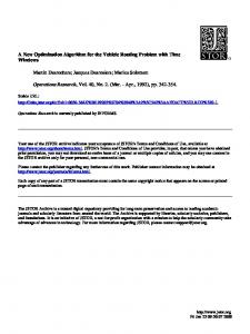
is valid for GRP(G). Like connectivity inequalities, R-odd cut inequalities induce facets of GRP(G) if and only if the subgraphs induced by S and V \ S are connected [5,6]. 2.4. K -C inequalities In order to present the remaining inequalities, we will need some more definitions. Consider the (generally disconnected) subgraph of G obtained by deleting all nonrequired edges from G. We call a connected component of this subgraph an R-connected component. A set of vertices defining an R-connected component will be called an R-set. An R-set with only one member will be called an isolated vertex. The K -Component or K -C inequalities [5,6] are defined in terms of an associated K -C configuration. A K -C configuration is (see Fig. 1) a partition {V0 , . . . VK } of V , with K ≥ 3, such that • V1 , . . . VK −1 and V0 ∪ VK are clusters of one or more R-sets, • |E R (V0 : VK )| is positive and even, • E(Vi : Vi+1 ) = ∅ for i = 0, . . . , K − 1. |E|

Given such a K -C configuration, consider a vector x ∗ ∈ R+ such that x ∗ (E(Vi : Vi+1 )) = 1 for i = 0, . . . ,K−1, but such that x ∗ (E(Vi : V j )) = 0 for all other 0 ≤ i < j ≤ K . Even if x ∗ is integral and satisfies all connectivity and R-odd cut inequalities, it still cannot represent a tour because x ∗ (δ(V0 )) and x ∗ (δ(VK )) should both be even. The main purpose of the K -C inequality is to cut off such ‘bad’ vectors x ∗ . The inequality takes the form: F(x) =

K −1 

x(δ(V0 ∪ · · · ∪ Vi )) − 2x(E(V0 : VK )) ≥ 2(K − 1).

(5)

i=0

K -C inequalities induce facets of GRP(G) when certain mild connectivity assumptions are met [5,6].

xP P  PPPxV  x  V1

V0

VK

2

Px PPP xV Px

3

VK −1

Fig. 1. K-C configuration

A cutting plane algorithm for the General Routing Problem

295

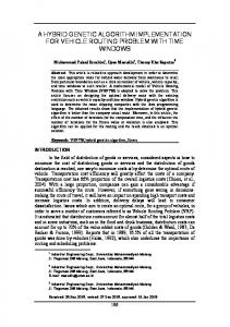
2.5. Path-bridge inequalities The path-bridge (PB) inequalities [19] are a generalization of K -C inequalities. They are defined in terms of an associated path-bridge (PB) configuration. Suppose p ≥ 1 and b ≥ 0 are integers such that p + b ≥ 3 and odd. Let n i ≥ 2 for i = 1, . . . , p also be integers. A PB configuration is (see Fig. 2) a partition of V into vertex sets A, Z and V ji for i = 1, . . . , p, j = 1, . . . , n i with the following properties: • • • •

each V ji is a cluster of one or more R-sets, |E R (A : Z )| = b, E(A : V1i ) = ∅ and E(Vni i : Z ) = ∅ for i = 1, . . . , p, i )  = ∅ for i = 1, . . . , p and j = 1, ..., n − 1. E(V ji : V j+1 i

The edges in E R (A : Z ) constitute the bridge. When b = 0, the bridge is empty and the PB configuration reduces to a path configuration, see [7]. In such a case, either or both of A and Z are permitted to be empty. For simplicity of notation, let us identify A with V0i and and Z with Vni i +1 for |E|

i = 1, . . . , p. Suppose that A and Z are non-empty. Consider a vector x ∗ ∈ R+ i )) = 1 for i = 0, . . . , p and j = 1, ..., n , but such that such that x ∗ (E(V ji : V j+1 i x ∗ (E(V ji : Vmk )) = 0 for all other quadruples i, j, k, m with 1 ≤ i, k ≤ p, 0 ≤ j ≤ n i +1 and 0 ≤ m ≤ n k . Even if x ∗ is integral and satisfies all connectivity and R-odd cut inequalities, it still cannot represent a tour. This is because x ∗ (δ(A))+b and x ∗ (δ(Z ))+b are both currently odd, whereas they should both be even. The main purpose of the PB inequality, at least when A and Z are non-empty, is to cut off such ‘bad’ vectors x ∗ . The formula for the coefficients in the PB inequality is rather complicated. However, our separation algorithms (Subsects. 3.5 and 3.6) are designed for so-called n-regular PB inequalities, in which all of the n i are equal to the same value n [7,19]. For such inequalities, there is a nice description of the coefficients in terms of vertex sets called handles and teeth. There are n − 1 handles, denoted by H1 , . . . , Hn−1 , and p teeth, p denoted by T1 , . . . , T p (see Fig. 3). The first handle is defined as H1 = A∪V11 ∪. . .∪V1 ; p 1 the other handles are defined inductively as Hi = Hi−1 ∪ Vi ∪ . . . ∪ Vi . The teeth are

V11

x P x PPPPxV

V21

x

A

V31

2 1

xV

2 2

Px PPP xV Px

2 3

Z

Fig. 2. PB configuration

296

Angel Corberán et al.

$ ' ' $  Px PP   PPx x  & % x x & % Px PPP x

Px H2 H1

T1

T2

Fig. 3. Handles and teeth in a 3-regular PB configuration

j

j

defined as T j = V1 ∪ . . . ∪ Vn . The n-regular PB inequality is then: n−1 

x(δ(Hi )) +

i=1

p 

x(δ(T j )) ≥ n p + n + p − 1

(6)

j=1

and is valid for GRP(G). Using the same techniques as in [7], it can be shown to be facet-inducing under mild connectivity assumptions. For brevity, we will call n-regular PB inequalities n-PB inequalities (where n may or may not be specified). Certain special cases of n-PB inequalities are of note. When p = 1, a K -C inequality is obtained. When b = 0, a regular path inequality is obtained [7]. The 2-PB inequalities are analogous to the well-known comb inequalities for the STSP (see, e.g., [13]). Finally, a 2-PB inequality in which each tooth consists merely of two isolated vertices (connected by a non-required edge) is called simple [19]. Simple 2-PB inequalities are analogous to the 2-matching inequalities for the STSP [13]. Note that simple 2-PB inequalities are not defined when the GRP instance is an RPP instance, because then there are no isolated vertices.

2.6. Honeycomb inequalities The honeycomb inequalities [6], like PB inequalities, are also a generalization of K -C inequalities. However, the generalization is in a different direction and neither class contains the other. A honeycomb configuration is a partition of V into sets Si such that: • for all i, | δ(Si ) \ δ R (Si ) |= ∅ and | δ R (Si ) | is even or zero; • there are at least two values i such that δ R (Si ) = ∅; • there are at least two values i such that δ R (Si ) = ∅; together with a set of non-required edges crossing between the Si which form a tree spanning the Si .

A cutting plane algorithm for the General Routing Problem

CxC C CC

x

V1

V2

 x

W1

V3

 

W2

W3

x

xW

@ ; @@Vx Vx;; 1

W3

2

2

x xV ; @ ; @@x x; W V3

Cx x x W1

297

4

4

Fig. 4. Two suitable honeycomb configurations

Many, but not all, honeycomb configurations can be formed by ‘gluing’ K -C configurations together by identifying edges [6]. In general, honeycomb configurations can be extremely complicated and computing the coefficients in the associated honeycomb inequality can be a formidable task. For this reason, we restrict ourselves in this paper to honeycomb configurations with a special structure. These consist of: • a partition {V1 , . . . , VL , W1 , . . . , W K −1 } of V , with L ≥ 2, K ≥ 3, such that (V1 ∪ . . . ∪ VL ), W1 , . . . , W K −1 are clusters of one or more R-sets, δ(Vi ) contains a positive and even number of required edges for all i and the graph induced by the required edges on the vertex set {V1 , . . . , VL } is connected. • a tree T spanning the sets V1 , . . . , VL , W1 , . . . , W K −1 such that the degree in T of every vertex set Vi is 1, the degree of vertex sets W j is at least 2 and the path in the tree connecting any distinct Vi , V j is of length 3 or more. If L = 2 the tree degenerates to a mere path and we have a K -C configuration. If L ≥ 3, then K ≥ 4 is needed in order for the path in the tree connecting any distinct Vi , V j to be of length 3 or more. Figure 4 shows two suitable honeycomb configurations. The bold lines represent edges in δ R (Vi ) for some i and the thin lines represent edges in the spanning tree. |E| Consider a vector x ∗ ∈ R+ such that: • x ∗ (E(Vi : V j )) = 0 for 1 ≤ i < j < L; • x ∗ (E(Vi : W j )) = 1 if and only if there is an edge connecting Vi and W j in the spanning tree, 0 otherwise; • x ∗ (E(Wi : W j )) = 1 if and only if there is an edge connecting Wi and W j in the spanning tree, 0 otherwise. Even if x ∗ is integral and satisfies all connectivity and R-odd cut inequalities, it still cannot represent a tour. This is because x ∗ (δ(Vi )) is odd for i = 1, . . . , L, whereas it should be even. The main purpose of the honeycomb inequality is to cut off such ‘bad’ vectors x ∗ . For honeycomb configurations with the special structure mentioned above, the coefficient αe of edge e ∈ E in the associated honeycomb inequality is equal to the number of edges traversed (if any) in the spanning tree to get from one end-vertex of e to the

298

Angel Corberán et al.

other, except for the edges with one end-vertex in Vi and the other in V j , i = j, when the coefficient is 2 units less. The honeycomb inequality is then:  αe x e ≥ 2(K − 1) (7) e∈E

These honeycomb inequalities define facets of GRP(G) if certain mild connectivity assumptions are met [6]. The right-hand sides of the honeycomb inequalities for the configurations shown in Fig. 4 are 6 for the configuration on the left and 8 for the configuration on the right. 3. Separation algorithms 3.1. Preliminary comments In this section, separation algorithms are presented for the inequalities described in the previous section. Before proceeding, however, we will need some definitions. |E| Given an LP relaxation vector x ∗ ∈ R+ , define the weighted graph G ∗ (V, E, x ∗ ). This weighted graph is input to all of the separation procedures. Given a graph G(V, E), a cut-vertex is a vertex the removal of which causes G to become disconnected. A block is a maximal connected subgraph of G which contains no cut-vertices. If a block consists of a single edge, then it is called a cut-edge. A decomposition of G into blocks can be found in O(|E|) time using the algorithm in [29]. We will also need the concept of shrinking a set of vertices in a weighted graph (see, e.g., [10,26]). Given a graph G(V, E) with weights on the edges, and a set W ⊂ V , shrinking W means identifying the vertices in W, deleting any resulting loops and merging each resulting set of parallel edges, if any, into a single edge. When merging parallel edges, the new edge is given a weight equal to the sum of the original weights. Shrinking can be done iteratively and, in the case of the GRP, a single edge in the shrunk graph can represent a mixture of any number of required or non-required edges in the original graph. In the following subsections, we describe heuristic (and sometimes exact) separation algorithms for each of the classes of inequalities described in the previous section. Some of the heuristics require the choice of a parameter (called ), or even two parameters (called 1 , 2 ). For details on which values of (or 1 , 2 ) we use and how the exact and heuristic algorithms are embedded in the overall algorithm, see Subsect. 4.2. 3.2. Connectivity separation Connectivity inequalities can be separated exactly in polynomial time. This is done by finding a minimum weight cut in the shrunk graph G s = (Vs , E s , x¯ ∗ ) obtained from G ∗ by shrinking each R-set into a single vertex. A minimum weight cut in an undirected graph with n vertices and m edges can be found in O(nm + n 2 log n) time using the algorithm in [21].

A cutting plane algorithm for the General Routing Problem

299

A faster (O(|E|) time) heuristic algorithm is obtained by computing the connected components of the subgraph induced by the edges e ∈ E s with x¯ e∗ > , where is a given parameter. Let S1 , S2 , . . . , Sq be the sets of vertices in the original graph G corresponding to the vertex sets of these connected components. Then x(δ(Si )) ≥ 2 is a violated connectivity inequality if q > 1 and x ∗ (δ(Si )) < 2. Note that when q = 2 we have x(δ(S1 )) = x(δ(S2 )), but when q > 2 all of the inequalities are distinct. 3.3. R-odd cut separation R-odd cut inequalities can also be separated exactly in polynomial time. Before describing the exact algorithm, however, we describe an effective separation heuristic. As for the connectivity inequalities, we choose a parameter . We compute the vertex sets S1 , S2 , . . . , Sq of the connected components of the subgraph of G ∗ induced by the edges e ∈ E with x e∗ > . Then x(δ(Si )) ≥ 1 is a violated R-odd cut inequality if q > 1, |δ R (Si )| is odd and x ∗ (δ(Si )) < 1. This heuristic runs in O(|E|) time and is inspired by a heuristic presented in [12] for blossom inequalities in the context of the perfect matching problem. The exact algorithm is much slower and involves finding a minimum weight R-odd cutset in G ∗ . Using a result of [25], this can be reduced to a series of maximum flow problems on G ∗ . The number of maximum flow computations needed in the worst case is equal to the number of R-odd vertices in G minus 1 and an R-odd cut inequality is violated if and only if the weight of the cutset is less than 1. As noted in [26] (in the context of the STSP), the idea of connected components can also be used to simplify the problem of finding an odd cut of weight less than 1. Consider the connected components of the subgraph of G ∗ induced by the edges e ∈ E with x e∗ > 0. Under the assumption that the separation heuristic has already been (unsuccessfully) invoked with = 0, we know that each of these components contains an even number of R-odd vertices. It is easy to show that we can examine each of these components independently for an odd cut of weight less than 1. This typically leads to considerable speed improvements in the exact algorithm. 3.4. K -C separation A vertex v ∈ V will be called R-odd if |δ R ({v})| is odd, otherwise it will be called R-even. Isolated vertices are R-even. It is not known if the problem of separating K -C inequalities can be solved in polynomial time or not, but our guess is that this problem is N P-hard. However, we have designed a heuristic algorithm which appears to work very well. It has three consecutive phases. In phase I, we find ‘seeds’ for V0 and VK . In phase II, we use these seeds to determine the Vi for i = 0, . . . , K . In phase III, we check the resulting inequality for violation, and, if it is not violated, we also check some other inequalities for violation which are obtained by shrinking the K -C configuration appropriately.

300

Angel Corberán et al.

x

@ x

@ @

{u} xP P

PPPx

@@ x @x 

Fig. 5. Getting seeds for V0 and VK

The details of these three phases are based on the following considerations: • We have examined the structure of the solutions obtained when all the connectivity and R-odd cut inequalities are satisfied. The effect of the K -C inequalities is to separate solutions x ∗ where an R-even vertex u belonging to an R-set Ci with |Ci | > 2 satisfies x ∗ (δ({u})) ∼ = 1 and x ∗ (E({u} : Ci \ {u})) ∼ = 0. Thus, {u} and Ci \ {u} are suitable vertex sets to be considered as seeds for V0 and VK , respectively, in phase I. Figure 5 illustrates this idea: the bold lines represent the required edges in E(Ci ) and the narrow lines represent non-required edges with x e∗ = 1. This idea is generalized by considering as seeds for V0 any vertex sets with an even number of R-odd vertices forming an x ∗ -connected component on the subgraph induced by Ci . • Given the seeds for V0 and VK , consider the graph obtained from G ∗ by shrinking the seeds and the remaining R-sets into a single vertex each. In order to define V0 , . . . , VK , we have to find a path in the shrunk graph connecting the seeds (preferably one with a large x ∗ -weight). Once this is done, we merely have to assign any vertices which are not in the path to one of the vertices in the path in order to complete phase II. • Suppose that a K -C inequality with K ≥ 4 is not violated. For i = 0, 1, 2, . . . , K −1, let L HS(i) = x ∗ (δ(V0 ∪ . . . ∪ Vi )). For some 1 ≤ i ≤ K − 2, we could merge sets Vi , Vi+1 into a single set, yielding a new ‘smaller’ (K -1)-C configuration, with an associated (K -1)-C inequality. From equation (5), for a given x ∗ , the slack of the new inequality will be equal to that of the original inequality, plus 2 − L HS(i). Thus, iteratively merging sets Vi , Vi+1 with L HS(i) > 2 will lead to inequalities with smaller slack, as long as K ≥ 3 remains. Alternatively, consider what would happen if we were to merge sets V0 , . . . , Vs into a
single set for some s ≤ K − 3. The resulting change in slack would be 2s − si=1 (L HS(i − 1) + 2x ∗ (Vi : VK )). Then, if this quantity was negative, the slack would have been reduced by shrinking. A similar argument applies if we merge sets Vt , . . . , VK for some t ≥ 3. It can also be shown that a K -C inequality cannot be violated if x ∗ (E(V0 : VK )) ≥ 1 and x ∗ satisfies all connectivity and R-odd cut inequalities. These are the ideas behind phase III. In our computer code, a given K -C configuration is stored by simply labelling each vertex in the graph according to the set Vi of the K -C configuration it belongs to. Computing coefficients from these labels is a simple matter and so is the operation of merging two or more Vi into one.

A cutting plane algorithm for the General Routing Problem

301

Taking into account the above points, the global procedure is as follows: • Phase I: Define seeds for V0 and VK . Given a specified R-set Ci , we say that a vertex in Ci is x ∗ -external if it is connected to at least one vertex in a different R-set by an edge e with x e∗ > 0. For each R-set Ci with at least two x ∗ -external vertices and connected to at least two different R-sets, do the following. Choose a parameter and construct the subgraph of G(Ci ) induced by edges e with x e∗ > . Look for an x ∗ -external vertex u whose corresponding connected component in the subgraph has an even number of R-odd vertices. If one is found, the connected component is a candidate for V0 and the complementary set in Ci is a candidate for VK (if VK = ∅). • Phase II: Define the vertex sets V0 , . . . , VK . Given the seeds for V0 and VK , we proceed as follows: (a) construct the graph obtained from G ∗ by shrinking the seeds and the remaining R-sets into a single vertex each. (b) Compute a spanning tree by iteratively adding the edge of maximum weight not forming a cycle (and not connecting the seeds). If this is not possible (because the removal of Ci disconnects the graph), then move on to another x ∗ -external vertex. (c) Transform the tree into a path linking the seeds, by (iteratively) shrinking each non-seed vertex with degree one into its (unique) adjacent vertex. If the length of the path is only 2, then move on to another x ∗ -external vertex. Otherwise, the vertices of the path define the vertex sets V0 , V1 , . . . , VK . Note that the seeds may have been enlarged in this process and therefore that either or both of V0 and VK may contain vertices from more than one R-set. • Phase III: Check the K -C inequality. We now have a K -C configuration like that of Fig. 1. For each
i = 0, 1, . . . , K − 1, compute L HS(i) = x ∗ (δ(V0 ∪ . . . ∪ Vi )). Then, K −1 ∗ L HS(i) − 2x ∗ (V0 , VK ) is the left hand side of the corresponding F(x ) = i=0 K -C inequality computed on x ∗ . If F(x ∗ ) < 2(K − 1), the K -C inequality is violated. If the K -C inequality is not violated, check if a violated inequality could be obtained by shrinking the K -C configuration. – Shrink all pairs Vi , Vi+1 with L HS(i) > 2, 1 ≤ i ≤ K − 2 and reduce K accordingly. If K < 3, stop (no violated inequality was found). – Compute the values: a = L HS(0) + 2x ∗ (E(V1 : VK )) − 2 b = L HS(K − 1) + 2x ∗ (E(V0 : VK −1 )) − 2 c = a + b + 2x ∗ (E(V1 : VK −1 )) corresponding to the reductions in slack which would be obtained if we shrank, respectively, the pair V0 , V1 or the pair VK −1 , VK , or both pairs simultaneously. If max{a, b, c} is larger than the slack, then shrink the pair V0 , V1 and/or the pair VK −1 , VK (depending on where the maximum of {a, b, c} is reached), to obtain a violated K -C inequality (if K ≥ 3 remains). – If this fails, it may yet be possible to obtain a violated inequality by shrinking. Compute for every 0 ≤ s, t ≤ K − 3, s + t ≤ K − 3, the reduction in slack (denoted by Ast ) which would be obtained if we shrank sets V0 , V1 , . . . Vs and sets VK , VK −1 . . . VK −t into single sets (this can be done quickly if the computations

302

Angel Corberán et al.

are performed in an intelligent way). If Ast > slack for any s, t such that K ≥ 3 would remain after shrinking, then select the s, t which gives the inequality with greatest violation. For a fixed value of , the algorithm looks for only one violated K -C inequality associated to each R-set. For each R-set Ci , priority is given to single vertices in Ci as candidates for V0 . Only if this fails to yield a violated inequality for the given Ci are more complex candidates for V0 considered. A simple extension of the heuristic allows us to search for violated K -C inequalities where the required edges in E(V0 : VK ) belong to more than one R-connected component. This is done by (iteratively) joining a pair of R-sets adjacent in G ∗ and then applying the above procedure as if they formed a single R-set.

3.5. n-PB separation: the case n = 2 When considering the separation of n-PB inequalities, it is useful to give the 2-PB inequalities special attention. Accordingly, the present subsection is concerned with 2-PB inequalities, whereas general n-PB inequalities are dealt with in the following subsection. In [19] it was shown, using ideas in [25], that the simple 2-PB inequalities can be separated exactly in polynomial time, provided that two conditions are met: • x ∗ satisfies all non-negativity and R-odd cut inequalities, • x ∗ (δ(e)) + x e∗ ≥ 3 holds for each e ∈ E. The first condition is obviously no problem. As for the second condition, it is easy to show that it is satisfied whenever x ∗ satisfies all connectivity inequalities. There are however two problems with the simple 2-PB separation algorithm. First, it is rather slow as it involves the computation of a minimum weight odd cut in a graph with O(|E|) vertices and O(|E|) edges. This problem can be alleviated to some extent by using the idea of connected components, as outlined in Subsect. 3.3. The second problem is that there are likely to be very few violated simple 2-PB inequalities, if any, when the GRP instance has few isolated vertices. Indeed, simple 2-PB inequalities are not defined at all for RPP instances. One way of improving the simple 2-PB separation algorithm would be to find conditions under which G ∗ can be shrunk (see Subsect. 3.1) in such a way that • A 2-PB inequality is violated in the shrunk graph if and only if a 2-PB inequality is violated by x ∗ , • A violated simple 2-PB inequality in the shrunk graph can be ‘expanded’ into a (not necessarily simple) 2-PB inequality violated by x ∗ . Although this idea has been applied successfully to related separation problems (see [10, 26]), we did not use it here because it turned out to be very difficult to devise appropriate data structures to account for the presence of required edges. A different idea was used instead.

A cutting plane algorithm for the General Routing Problem

303

Consider the graph G ∗ obtained from G ∗ by deleting non-required edges e with = 0. Suppose we have a block decomposition of G ∗ (see Subsect. 3.1) and that there are h ≥ 2 blocks. Let V( j) for j = 1, . . . , h denote the set of vertices in block j, let G j for j = 1, . . . , h denote the subgraph of G ∗ induced by V( j) and let x( j) denote the vector obtained from x ∗ by dropping all components apart from those corresponding to edges in E(V( j)). It is possible to show that a 2-PB inequality is violated by x ∗ if and only if there is at least one j such that a 2-PB inequality (valid for GRP(G j )) is violated by x( j). We therefore apply the simple 2-PB algorithm to each G j separately. If a violated simple 2-PB inequality is found for some G j , we expand it into a (not necessarily simple) 2-PB inequality violated by x ∗ . This is done by viewing G j as being obtained from G ∗ by shrinking, in any order, those V(i) such that i = j. This approach typically yields considerable speed improvements, because it is frequently the case that there are h ≥ 2 blocks. Moreover, it typically leads to more violated inequalities being discovered. x e∗

To avoid difficulties due to rounding errors, we actually define G ∗ a little differently: we delete from G ∗ all non-required edges e with x e∗ < 0.01. 3.6. n-PB separation: the general case The separation of n-PB inequalities appears to be very difficult and is likely to be N Phard. However, the authors have devised a separation heuristic which is fast (it can be implemented to run in O(|V |.|E|. log |V |) time) and quite effective. In fact, it has proved worthwhile to run this heuristic before the heuristic for 2-PB inequalities described in the previous subsection. Like the 2-PB heuristic, the n-PB heuristic is applied to each block G j of G ∗ separately and each resulting violated inequality is ‘expanded’ to yield an inequality violated by x ∗ . From now on we assume that we are working on an individual block, but for simplicity of notation we assume that there is in fact only one block, the graph G ∗ itself. Given any two R-sets S1 , S2 connected by at least one edge, let θ(S1 , S2 ) = x ∗ (δ(S1 ∪ S2 )) + x ∗ (E(S1 : S2 )) − 3. It can be shown that, when all connectivity inequalities are satisfied, then θ(S1 , S2 ) ≥ 0. In limited experiments, adjacent pairs V ji i and V j+1 in violated n-PB inequalities often turned out to be R-sets S1 , S2 such that θ(S1 , S2 ) was small. This fact is used in the first stage of the heuristic, which is to get a good set H of candidates for H1: • Choose two parameters 0 ≤ 1 , 2 ≤ 1. • Initially all edges are unlabelled. • Examine each pair S1 , S2 of R-sets connected by at least one edge. If θ(S1 , S2 ) ≤ 1 , then label the edges in E(S1 ) and E(S2 ) ‘strong’ and the edges in E(S1 : S2 ) ‘weak’. Store (S1 , S2 ) as a ‘candidate tooth’. S1 and S2 are the ‘ends’ of the candidate tooth. • Examine the remaining unlabelled edges. Label such an edge e ‘weak’ if x e∗ ≤ 2 . • Delete all weak edges from G ∗ . • Examine each connected component in the resulting graph. Let C be the set of vertices in one such component. Let b = |δ R (C)| and let p equal the number of candidate teeth with exactly one end in C. If p + b ≥ 3 and odd, p ≥ 1 and the p candidate teeth mentioned are vertex-disjoint, then put C into the list H of candidates for H1.

304

Angel Corberán et al.

It is possible to implement this to run in O(|E|) time, by first of all computing x ∗ (δ(S)) for each R-set S. Notice also that, for fixed 1 , 2 , |H| is O(|V |). The remainder of the heuristic is repeated for each candidate H1 ∈ H. First, we check whether the simple 2-PB inequality with handle H1 and the p candidate teeth is violated. If so, we store this violated inequality. Whether or not this simple 2-PB inequality is violated, we then proceed to look for a more general n-PB inequality which is violated. p To this end, we set V11 , . . . , V1 to be the ends of the p candidate teeth lying in H1. The remainder of H1, if any, is used to form A. The other ends of the p candidate teeth p are used to form ‘seeds’ for V21 , . . . , V2 . We then construct a shrunk graph from G ∗ as follows: • Shrink the R-sets which are contained entirely in H1 into a single vertex each, and do the same for the R-sets which are contained entirely in V \ H1. • Shrink the vertices in H1 which are incident on one or more crossing required edges into a single ‘inner pole’ vertex (unless there are no such vertices). • Shrink the vertices in V \ H1 which are incident on one or more crossing required edges into a single ‘outer pole’ vertex (unless there are no such vertices). Let G s (Vs , E s , x¯ ∗ ) denote the weighted shrunk graph and let Hs denote the shrunk H1. In the next stage, G s is used to enlarge the PB configuration. We distinguish two cases. • Case 1: b ≥ 1. Here, A is non-empty and we also have an obvious ‘seed’ for Z; namely, the outer pole. If x¯ ∗ (E(A : Z )) ≥ 1, we give up. Otherwise we follow a similar idea to that used in the K -C heuristic: we iteratively add edges in order of non-increasing weight so as to build a tree in G s with the following properties: – It spans all vertices in Vs apart from those representing A and the V1i . – It consists of p + 1 edge-disjoint subtrees. – Subtree i for i = 1, . . . , p contains a path from the V2i seed to the Z seed but does j not contain any paths from the V2i seed to any other V2 seed, j = i. – Subtree p + 1 (which may be empty) connects the Z seed to other vertices, but does not contain any paths from Z to any of the V2i seeds. Once the structure has been made, we iteratively shrink vertices of degree one (different from the V2i and Z seeds) into their unique adjacent vertex to obtain a (not necessarily regular) PB configuration. • Case 2: b = 0. Here, p ≥ 3, it is possible for A to be empty and we do not have a ‘seed’ for Z. We build two structures, one in which Z is forced to be empty and one in which Z is forced to non-empty. In the first case, we build a forest in G s which spans all vertices in Vs apart from those representing A and the V1i . It must consist of p vertex-disjoint trees, such that each of the V2i seeds is contained in exactly 1 tree. Once the forest is made, we pick longest paths going out from each of the V2i seeds to get the p necessary paths and shrink vertices of degree 1 as before. In the second case, we build a tree in G s which spans all vertices in Vs apart from those representing A and the V1i . Now, an edge is permitted to create a path connecting two distinct V2i seeds. Once this happens, one of the vertices on the path (different

A cutting plane algorithm for the General Routing Problem

305

from the V2i seeds) must now be a Z seed. The remainder of the tree is built with this in mind: The addition of an edge forming a path connecting one of the possible Z seeds to a third V2i seed is not permitted unless it is incident on a potential Z seed (which is then chosen as the actual Z seed). If this never happens (because the shrunk graph is not sufficiently connected), the tree is abandoned. Otherwise, we proceed as in Case 1 now that we have our Z seed. At this stage, we will generally have a non-regular PB configuration (or possibly two). Moreover, the structure of the configuration in the vicinity of Z is likely to be ‘messy’. We deal with both of these problems simultaneously: We choose n according to the length of the shortest of the p paths in the configuration and shrink any paths which are longer than this by merging Z with adjacent V ji . Now that we have an n-PB inequality, we check if is violated. If not, we may still be able to obtain a violated inequality by ‘removing handles’ (analogous to shrinking a K -C configuration). It is easy to see from the inequality (6) that the slack of the n-PB inequality will be decreased by removing any handle Hi such that x ∗ (δ(Hi )) > p + 1 and merging adjacent V ji accordingly. This is done iteratively, as long as n ≥ 2 remains.

3.7. Honeycomb separation As for the K -C inequalities, we first try to separate honeycomb inequalities in which a single R-connected component is partitioned into more than 2 parts. The effect of these honeycomb inequalities is to separate solutions x ∗ where some R-even vertices u 1 , u 2 , . . . , u L (or sets with an even number of R-odd vertices) belonging to an R-set Ci satisfy x ∗ (δ(u j )) ∼ = 1 and x ∗ (E({u j } : Ci \ {u j })) ∼ = 0, j = 1, 2, . . . , L. The idea of our algorithm is, given an R-connected component, to find the x ∗ external vertices, say u 1 , u 2 , . . . , u t , and, then, assign the remaining vertices to some of the previous ones in order to define vertex sets V1 , V2 , . . . , Vt in such a way that x ∗ (E(Vi : V j )) is as small as possible, for 1 ≤ i < j ≤ t. The procedure is as follows: Phase I: Define seeds for V1 , V2 , . . . , VL . Given an R-set Ci , we assign to each x ∗ -external vertex u j a label k corresponding to the R-set C k with x ∗ ({u j } : C k ), k = i maximum. To each of the remaining vertices in Ci , a different negative label is assigned. Starting with the edge (u, v) in E(Ci ) with largest x ∗ -weight, let lmin (lmax ) be the smaller (larger) label of that of u and v. We assign the label lmax to all vertices in Ci having label lmin . This procedure is repeated until all vertices have positive label. Vertices with the same label define a partition V1 , V2 , . . . , Vt of the set of vertices of Ci . If the number of R-odd vertices in each V j , j = 1, . . . , t is even, we are done. Otherwise, all the sets V j with an odd number of R-odd vertices are joined, forming a single set. Hence, we have defined a partition V1 , V2 , . . . , VL . If L ≥ 3, these sets are suitable to be considered as part of a honeycomb configuration. If L = 2, these sets are suitable to be considered as V0 and VK for a K -C configuration. Since this way

306

Angel Corberán et al.

of defining V0 and VK is different from that of Phase I in the above K -C separation algorithm, it is worthwhile to look for a violated K -C inequality. We then apply Phases II and III of K -C separation. Otherwise (L = 1), we study another R-connected component. Phase II: Define the vertex sets W1 , W2 , . . . , W K −1 and the tree. After (seeds for) V1 , V2 , . . . , VL have been defined, we consider the graph obtained by shrinking each V1 , V2 , . . . , VL and each of the remaining R-sets into single vertices. As in the separation of K -C and n-PB inequalities, we try to compute a spanning tree with large x ∗ weight in this shrunk graph, by iteratively adding the edge of maximum weight not forming a cycle (and not crossing between the Vi ). Initially we forbid adding edges of zero weight. If we obtain a tree without having to add an edge of zero weight, we then shrink (iteratively) each vertex with degree one on the tree (different from V1 , V2 , . . . , VL ) into its (unique) adjacent vertex, thus obtaining the vertex sets W1 , W2 , . . . , W M and the tree defining the honeycomb configuration. If we do not, then before adding edges of zero weight, we check each one of the connected components in the forest to see whether it defines a honeycomb configuration by itself. Only if this also fails do we add to the forest the edges of zero weight needed to get a spanning tree. If the degree of any vertex Vi on the tree is more than two, we reject that honeycomb configuration and consider another R-connected component. Otherwise, for each vertex Vi incident with two vertices, W j and Wk , on the tree, we replace one of the edges (Vi , W j ) or (Vi , Wk ) (that with largest x ∗ -weight) by edge (W j , Wk ) on the tree. Then, every vertex Vi has degree one in the configuration tree. If the above procedure has been successful, we now have a honeycomb configuration defined by V1 , V2 , . . . , VL and W1 , W2 , . . . , W K −1 and its corresponding inequality F(x) ≥ 2(K − 1). Phase III: Check the Honeycomb inequality. For a given vector x ∗ , in order to compute F(x ∗ ), we define a vector with a record T(e) for each edge in the configuration tree. For each edge e ∈ E, we add x e∗ to the records corresponding to the edges in the (unique) path on the tree joining the two ‘shrunk’ vertices containing the two end-vertices of edge e. Then, we can compute easily   F(x ∗ ) = T(e) − 2 x ∗ (Vi : V j ) (8) e∈T

1 10, stop. K -C separation heuristic with = 0, 0.25, 0.5. If the number of violated inequalities detected so far is > 15, stop. Else do honeycomb separation heuristic (that can also find K -Cs). 7. If the number of violated inequalities detected so far is > 15, stop. Else do n-PB heuristic with 1 = 0, 0.25, 0.5, 0.75 and 1 and 2 = min{0.25, 1}. 8. If the number of violated inequalities detected so far is > 5, stop. Else do heuristics for K -Cs and honeycombs with iterative merging of adjacent R-components. 9. If no violated inequality has been found so far, then do 2-PB heuristic (which is exact for simple 2-PBs).

1. 2. 3. 4. 5. 6.

308

Angel Corberán et al.

When E R = ∅ (i.e., when the GRP instance is a SGTSP instance), it is better to use the following strategy: 1. Connectivity separation heuristics with = 0, 0.25, 0.5. 2. If the number of violated inequalities detected so far is > 15, stop. Else do n-PB heuristic with 1 = 0, 0.25, 0.5, 0.75 and 1 and 2 = min{0.25, 1}. 3. If no violated inequalities have been detected so far (or, every fifth iteration, no connectivity inequalities have been found so far), do exact connectivity separation algorithm. 4. If no violated inequality has been found so far, then do 2-PB heuristic. 4.3. Constraint management and the cut pool When a large number of cuts have been added, the LPs can become rather large, causing speed and memory problems. To alleviate this problem, it is helpful to occasionally ‘purge’ constraints from the LP formulation. We found that a good strategy was to remove, every 10 iterations, any constraints which have a slack of 0.01 or more. However, it can happen that a constraint which was removed at one time can become violated in a subsequent iteration. Because of the heuristic nature of some of the separation algorithms, this could lead to a useful constraint being lost forever. To avoid this difficulty, we use the idea of a cut pool [27]. Every time a violated inequality is found, it is stored in the cut pool. Then, whenever the LP is purged, the cut pool is checked to see if it contains any violated constraints. If so, these are added to the LP and the LP is then re-solved. We also search through the cut pool whenever the separation algorithms fail to find a violated inequality. 4.4. Additional phase If no more violated inequalities can be found and the solution vector x ∗ still does not represent an optimal tour, we do some more things. First, we use a recent result in [11]. Consider the graph obtained by shrinking each Rset of G into a single vertex, but without merging parallel edges. Construct a minimum cost spanning tree T on this graph (using the ce as costs). Then there is an optimal solution to the GRP such that the following conditions hold: • x e ≤ 2 for all e ∈ T , • x e ≤ 1 for all e ∈ / T. These upper bounds dominate the ones mentioned in Subsect. 4.1. We insert these upper bounds into the LP relaxation and then call the separation procedures again. (The reason that we do not put these upper bounds in from the very start is that, on some instances, their presence can create spurious ‘odd’ vertices in the LP relaxation.) If this still does not yield the optimal tour and the lower bound is not an integer value, we append an extra inequality which enforces integrality of the objective and then call the separation procedures
again. (For example, if the lower bound was 100.23, then we would add the constraint e∈E ce x e ≥ 101.)

A cutting plane algorithm for the General Routing Problem

309

If, after all this, the LP relaxation is still not integral, we invoke branch-and-bound. To avoid the solution of very large integer programs (IPs), we first delete all constraints with a slack of 0.01 or more. We have found that the resulting IP is usually solved quickly and often leads to the optimal solution of the GRP. However, it is possible that the IP solution might not be feasible for the GRP, since the associated ‘tour’ could fail to be connected, Eulerian, or both. In such a case, the procedure terminates with a (very tight) lower bound, but no feasible GRP solution.

5. Computational experiments The algorithm has been coded in the C language and run on a SUN Sparc 20 workstation, using the CPLEX library to solve the LP problems. (Note that the SUN machine is rather slow. Its speed is comparable to a 66 MHz Pentium). The algorithm has been tested on RPP and GTSP instances, as well as ‘genuine’ GRP instances. A description of the test instances follows: • 24 RPP instances, denoted by I1 to I24, from [4] and two more RPP instances, denoted by IAA and IAB, from [5] obtained by randomly selecting some edges in the realworld based graph, with 116 vertices and 174 edges, of the city of Albaida (Valencia) (Table 1). • 92 RPP instances from [15]. In these problems, the vertices lie on the Euclidean plane and edge costs are proportional to Euclidean distances. The set E is formed according to one of three procedures and then the set E R is chosen randomly. In the first procedure (used for 20 instances, Table 2), E is made of edges with short length in the plane. In the second procedure, (used for 36 instances, Table 3), E forms a unit grid graph. In the third procedure (also used for 36 instances, Table 4), G is a graph in which all vertices have degree 4, made from two edge-disjoint Hamiltonian cycles found by a nearest neighbour heuristic. These instances have 16 ≤ |V | ≤ 100 and 24 ≤ |E| ≤ 200. • 10 GRP instances generated from the Albaida graph by visually selecting the required edges. We select, for example, edges corresponding to streets oriented from north to south, from east to west, forming cycles, etc. (Table 5). • 15 GRP instances randomly generated from the Albaida graph, by defining each edge as required with probability P and considering all the vertices of the graph as required. Five graphs were generated for each value of P = 0.7, 0.5 and 0.3, named alb-7-1 to alb-3-5 (Table 6). • 15 GRP instances, named mad-7-1 to mad-3-5, randomly generated from the realworld based graph of the city of Madrigueras (Albacete) — with 196 vertices and 316 edges — in the same way as for Albaida (Table 7). • 7 GTSP instances with between 150 and 225 vertices and between 296 and 433 edges (Table 8). These were formed by taking planar Euclidean TSP instances from TSPLIB [28] and making the associated graphs sparse by deleting all edges apart from – The edges in an optimal TSP tour – The edges connecting each vertex to its three nearest neighbours.

310

Angel Corberán et al.

For these instances, the cost of the optimal solution was known beforehand. Also, some of the edges in these instances could be eliminated using the criterion given in Subsect. 4.1. However, we only did this for the two largest instances (rat195g and ts225g). In the following tables, LB0 shows the lower bound values corresponding to the initial relaxations, while LB shows the lower bound values obtained at the end of the cutting-plane procedure. For the cases where branch and bound was used, the solution cost is given in the B&B column. Total running times have also been included. For each instance in Tables 1 and 5 to 8, the number of identified violated connectivity, R-odd cut, K -C, honeycomb, K -C and honeycombs with merging of adjacent R-sets, n-PB and simple 2-PB constraints are presented under headings conn, odd, K-C, HC, KC2, HC2, nPB and SPB, respectively. In all tables, a ‘*’ on a LB or B&B entry means that not only the optimal value but also an optimal GRP solution was obtained using the cutting-plane algorithm alone, or the cutting-plane algorithm plus B&B, respectively. A ‘*’ on an UB entry means that this upper bound is optimal. In Tables 2 to 4 the entries corresponding to the different types of constraints and to the running time represent the accumulated amount for all the instances in each group. Moreover, the number of instances in each group solved to optimality with cuttingplanes alone and the number of instances that were solved to optimality after B&B are shown. Finally, the upper bounds shown in Table 5 for instances grp4 and grp10 were obtained by Alain Hertz (private communication) using the methods in [15]. Instances grp4 and grp10 were built to be difficult, but it is our belief that both upper bounds should be optimal or very near optimal, as the sophisticated heuristic procedures of [15] produced optimal solutions for all the instances reported in Tables 1 to 4 and for the 8 other instances of Table 5. It will be seen that 116 out of 118 RPP instances were solved to optimality by cutting planes alone and the other 2 were solved after invoking branch and bound. The maximum percentage gap between the LP lower bound value and the optimal cost was 0.26% for these instances. Thus, the algorithm works extremely well for RPP instances. When it comes to ‘genuine’ GRP instances, it will be seen that 28 out of 40 instances were solved to optimality by cutting planes alone and a further 6 were solved by branch and bound. The maximum percentage gaps between the LP lower bound and the optimal cost or upper bound were 1.81% for instance grp10 in Table 5, 0.5% for instance alb-3-1 in Table 6 and 0.37% for instance mad-5-5 in Table 7. Finally, 3 out of the 7 GTSP instances, 6 if we resorted to branch and bound, were solved to optimality. The worst performance was obtained for the instance ts225g. For this instance, the percentage gap was 1.62%, and the branch-and-bound algorithm failed to find the optimal integer solution after 20,000 nodes had been explored. (Note, however, that the corresponding TSPLIB instance, ts225, was deliberately constructed to be difficult for cutting plane algorithms). It will also be noticed that the running times were somewhat larger for the GTSP instances than for the RPP and GRP instances. Even so, they are acceptable given that our machine is at least 8 times slower than a modern PC.

A cutting plane algorithm for the General Routing Problem

311

6. Conclusions The computational results given in the previous section show that our cutting plane algorithm is capable of solving many GRP instances of realistic size to proven optimality. This provides further evidence, if evidence were needed, that the study of integer polyhedra is important from a practical as well as a theoretical point of view. Of course, there is still room for improvement in our algorithm. One obvious improvement would be the addition of better separation algorithms. In this context, ‘better’ could simply mean faster, or it could mean generating more inequalities or inequalities of greater generality. Another improvement would be to embed the separation algorithms within a full branch-and-cut scheme (see [27]). Finally, we would also like to mention that the separation procedures presented in this paper could be useful for more complex routing problems, perhaps containing multiple vehicles, directed arcs or other complications encountered in practice (see [9] for a survey). Acknowledgements. The authors want to thank Alain Hertz for providing us his instances and upper bounds and José Manuel Belenguer for providing us with some useful code, such as the subroutine for computing minimum weight odd cuts. Thanks are also due to the anonymous referees for their comments.

References 1. Applegate, D., Bixby, R.E., Chvátal, V., Cook, W. (1995): Finding cuts in the TSP. DIMACS Technical Report TR 95–05, Rutgers University, New Brunswick, NJ, USA 2. Augerat, P., Belenguer, J.M., Benavent, E., Corberán, A., Naddef, D., Rinaldi, G. (1995): Computational results with a branch-and-cut code for the capacitated vehicle routing problem. Research report RR949–M, ARTEMIS-IMAG, France 3. Belenguer, J.M., Benavent, E. (1998): The capacitated arc routing problem: valid inequalities and facets. Comput. Optim. Appl. 10, 165–187 4. Christofides, N., Campos, V., Corberán, A., Mota, E. (1981): An algorithm for the rural postman problem. Imperial College Report IC.OR.81.5, London 5. Corberán, A., Sanchis, J.M. (1994): A polyhedral approach to the rural postman problem. Eur. J. Opl Res. 79, 95–114 6. Corberán, A., Sanchis, J.M. (1998): The general routing problem polyhedron: facets from the RPP and GTSP polyhedra. Eur. J. Opl Res. 108, 538–550 7. Cornuéjols, G., Fonlupt, J., Naddef, D. (1985): The travelling salesman on a graph and some related integer polyhedra. Math. Program. 33, 1–27 8. Edmonds, J., Johnson, E.L. (1973): Matchings, Euler tours and the Chinese postman problem. Math. Program. 5, 88–124 9. Eiselt, H.A., Gendreau, M., Laporte, G. (1995): Arc-routing problems, part 2: the rural postman problem. Oper. Res. 43, 399–414 10. Fleischmann, B. (1985): A cutting-plane procedure for the travelling salesman problem on a road network. Eur. J. Opl Res. 21, 307–317 11. Ghiani, G., Laporte, G. (2000): A branch-and-cut algorithm for the undirected rural postman problem. Math. Program. 87, 467–482 12. Grötschel, M., Holland, O. (1985): Solving matching problems with linear programming. Math. Program. 33, 243–259 13. Grötschel, M., Padberg, M.W. (1979): On the symmetric travelling salesman problem I: inequalities. Math. Program. 16, 265–280 14. Grötschel, M., Win, Z. (1992): A cutting plane algorithm for the windy postman problem. Math. Program. 55, 339–358 15. Hertz, A., Laporte, G., Nanchen, P. (1999): Improvement procedures for the undirected rural postman problem. INFORMS J. Comput. 11, 53–62

312

Angel Corberán et al.

16. Jünger, M., Reinelt, G., Rinaldi, G. (1995): The travelling salesman problem. In: Ball et al., eds., Network Models. Handbooks on Operations Research and Management Science Vol. 7. Elsevier, Amsterdam 17. Jünger, M., Reinelt, G., Rinaldi, G. (1997): The travelling salesman problem. In: Dell’Amico et al., eds., Annotated Bibliographies in Combinatorial Optimization. Wiley, New York 18. Lenstra, J.K., Rinnooy-Kan, A.H.G. (1976): On general routing problems. Networks 6, 273–280 19. Letchford, A.N. (1997): New inequalities for the general routing problem. Eur. J. Opl Res. 96, 317–322 20. Letchford, A.N. (1999): The general routing polyhedron: a unifying framework. Eur. J. Opl Res. 112, 122–133 21. Nagamochi, H., Ono, T., Ibaraki, T. (1994): Implementing an efficient minimum capacity cut algorithm. Math. Program. 67, 325–341 22. Nemhauser, G.L., Wolsey, L.A. (1988): Integer and Combinatorial Optimization. Wiley, New York 23. Nobert, Y., Picard, J.-C. (1996): An optimal algorithm for the mixed Chinese postman problem. Networks 27, 95–108 24. Orloff, C.S. (1974): A fundamental problem in vehicle routing. Networks 4, 35–64 25. Padberg, M.W., Rao, M.R. (1982): Odd minimum cut-sets and b-matchings. Math. Oper. Res. 7, 67–80 26. Padberg, M.W., Rinaldi, G. (1990): Facet identification for the symmetric travelling salesman polytope. Math. Program. 47, 219–257 27. Padberg, M.W., Rinaldi, G. (1991): A branch-and-cut algorithm for the resolution of large-scale symmetric travelling salesman problems. SIAM Rev. 33, 60–100 28. Reinelt, G. (1991): TSPLIB – a travelling salesman problem library. ORSA J. Comput. 3, 376–384 29. Tarjan, R.E. (1972): Depth first search and linear graph algorithms. SIAM J. Comp. 1, 146–60

A cutting plane algorithm for the General Routing Problem

313

Table 1. Computational results for the Christofides et al. (1981) and Corberán & Sanchis (1994) instances constraints |V |

Rsets

LB0

conn.

odd

K-C

KC2

HC

HC2

nPB

LB

time (scs.)

I01 I02 I03 I04 I05

11 14 28 17 20

4 4 4 3 5

31 62 24 24 49

5 4 5 3 5

10 10 16 14 14

4 9 7 14

4 9

-

-

-

51* 72* 29* 29* 55*

0.03 0.04 0.10 0.10 0.17

I06 I07 I08 I09 I10

24 23 17 14 12

7 3 2 3 4

27 35 26.5 18 27

8 3 2 3 5

24 18 16 12 10

13 1 8

6 -

-

-

-

32* 37* 29* 26* 35*

0.23 0.08 0.09 0.06 0.10

I11 I12 I13 I14 I15

9 7 7 28 26

3 3 3 6 8

9 6 23 43 207

3 3 3 9 16

6 6 6 28 30

2 18 2

6 1

-

-

-

9* 6* 23* 57* 261*

0.08 0.02 0.01 0.32 0.23

I16 I17 I18 I19 I20

31 19 23 33 50

7 5 8 7 7

53 39 54 112 80

8 7 12 7 12

25 16 26 30 34

14 9 3 26

3 6 8

6 2 1 3

1 1 2

2 -

64* 49* 85* 116* 116*

0.64 0.17 0.17 0.12 0.54

I21 I22 I23 I24

49 50 50 41

6 6 6 7

52 103 78 96

9 7 10 8

40 30 45 33

41 3 51 28

19 32 16

8 1 2 6

3 2 5

2 2

78* 122* 95* 113*

1.25 0.31 1.18 1.17

IAA IAB

102 90

10 11

2896 1728

11 17

114 87

105 11

90 4

15 4

15 2

3 -

3304* 2826*

6.98 2.42

Table 2. Computational results for Class 1 RPP random instances from Hertz et al. (1999) TOTAL constraints for all 5 instances n

# of inst.

R-sets average

conn.

odd

K-C

KC2

HC

HC2

20 30 40 50

5 5 5 5

3.4 4.8 7.0 8.2

18 30 46 59

44 80 107 130

2 24 31 13

13 17 10

2 4

1 2

nPB

# of LB opt.

# of B&B opt.

Total time (scs.) for all 5 instances

2 4

5 5 5 5

-

0.20 0.56 1.18 1.60

314

Angel Corberán et al.

Table 3. Computational results for Class 2 RPP random instances from Hertz et al. (1999)

R-sets average

TOTAL constraints for all 3 instances conn.

odd

K-C

KC2

HC

HC2

nPB

# of LB opt.

# of Total time B&B (scs.) for all opt. 3 instances

n

Prob.

# of inst.

16

0.3 0.5 0.7

3 3 3

4.0 4.3 4.0

13 13 14

26 28 30

2 19

2 6

-

-

-

3 3 3

-

0.11 0.11 0.21

36

0.3 0.5 0.7

3 3 3

8.3 6.6 5.6

33 24 22

72 96 91

45 46 64

28 23 34

2 9

2 6

1 -

3 3 3

-

1.00 1.22 1.28

64

0.3 0.5 0.7

3 3 3

12.0 9.0 5.0

57 35 21

137 51 226 102 151 80

22 43 26

3 14 -

2 9 -

4 1 -

3 3 3

-

2.75 9.19 2.97

100

0.3 0.5 0.7

3 3 3

19.6 14.0 6.3

86 72 35

243 97 43 28 977 571 312 154 528 281 107 66

12 81 24

9 3 -

3 2 3

1 -

16.56 109.11 42.38

Table 4. Computational results for Class 3 RPP random instances from Hertz et al. (1999)

R-sets average

TOTAL constraints for all 3 instances conn.

odd

K-C

KC2

HC

HC2

nPB

# of LB opt.

# of Total time B&B (scs.) for all opt. 3 instances

n

Prob.

# of inst.

16

0.3 0.5 0.7

30 3 3

3.0 3.6 4.6

10 13 16

24 26 34

6 4 8

2 2

-

-

-

3 3 3

-

0.09 0.19 0.22

36

0.3 0.5 0.7

3 3 3

8.3 7.3 5.3

30 25 20

72 74 106

20 29 31

12 19 8

-

-

-

3 3 3

-

0.59 0.79 0.96

64

0.3 0.5 0.7

3 3 3

12.3 10.3 6.6

45 43 23

122 49 273 106 192 69

34 57 40

3 13 7

2 6 4

1 6 3

3 3 3

-

2.04 8.61 3.46

100

0.3 0.5 0.7

3 3 3

20.3 13.0 9.0

93 61 38

325 93 275 82 348 151

57 26 57

5 14 32

4 4 4

4 5 -

3 3 2

1

21.79 8.08 23.61

A cutting plane algorithm for the General Routing Problem

315

Table 5. Computational results for 10 visually generated instances from the Albaida graph (116 vertices and 174 edges) constraints Rsets

LB0

conn.

56 52 55 48 45 10 64 47 60 48

4183 3748 3937 2576 3620 2568 4525 5044 3329 2480

84 87 90 114 68 13 103 85 93 121

grp1 grp2 grp3 grp4 grp5 grp6 grp7 grp8 grp9 grp10

odd

K-C

127 53 194 128 125 31 45 311 115 26 92 113 52 132 44 92 17 404

KC2

HC

HC2

nPB

LB

16 96 16 26 16 27 16 12 66

8 22 4 350 12 18 17 15 429

3 9 4 49 6 4 2 8 82

9 6 1 2 2 3 3 -

5625* 5569* 5688* 5119 5191* 3442* 6618* 6814* 4506* 5029

B&B

UB

5158

5186

5070

5122

time (scs.)

# of iter.

42.1 506.2 65.4 1155.5 118.6 1.3 109.9 31.5 206.9 2010.7

14 36 13 67 13 4 14 17 15 85

Table 6. Computational results for 15 randomly generated instances from the Albaida graph (116 vertices and 174 edges) constraints Rsets

LB0

7-1 7-2 7-3 7-4 7-5

18 10 15 10 13

2789 2538 2480 2456 2714

5-1 5-2 5-3 5-4 5-5

33 30 28 33 30

3-1 3-2 3-3 3-4 3-5

66 71 72 67 62

conn. odd

HC2

nPB

SPB

LB

24 10 20 11 15

242 100 84 3 122 3 1 2 178 242 225 36 190 155 22 21 3

1 31 3

2 -

2 -

4374* 3562* 3559* 3582* 4077*

106.2 3.0 33.0 20.2 30.9

63 14 43 49 34

3374 3219 3432 3140 3400

45 42 38 46 41

144 125 124 10 106 15 107 43 106 21

93 10 5 24 -

19 4 8 10 1

12 1 -

8 2 -

3 -

4785* 4641* 4322* 4714 4719* 4332*

84.8 26.0 13.0 101.9 6.2

24 9 11 23 8

4042 4666 4490 4165 4395

115 122 133 120 97

160 122 99 135 107

25 34 12 25 6

30 16 4 11 24

18 6 3 5 15

4 15 10 8 4

2 -

5703 5712 5732* 6699 6716* 6189 6189 6201* 5926* 5856*

276.8 194.4 192.3 138.8 147.0

29 25 20 25 13

56 57 22 84 26

KC2

B&B

UB

time # of (scs.) iter.

HC

K-C

316

Angel Corberán et al.: A cutting plane algorithm for the General Routing Problem

Table 7. Computational results for 15 randomly generated instances from the Madrigueras graph (196 vertices and 316 edges) constraints Rsets 7-1 15 7-2 6 7-3 11 7-4 7 7-5 8

LB0

conn. odd

K-C

KC2

HC

HC2

nPB

SPB

LB

4 -

-

-

5260* 4930* 5135* 4775* 5375*

B&B

UB

time (scs.)

# of iter.

11.0 7.8 9.8 9.4 9.0

10 11 10 14 17

4325 4520 4322.5 4047.5 4617.5

19 6 12 8 8

160 35 172 164 8 162 192 -

19 6 -

8 3 -

6010 5715 6160 5857 5900

51 57 73 82 70

206 172 222 228 204

100 17 104 180 39

92 73 64 16

14 3 3 8 25 14 5 79 25 12 10 - 5

-

6920* 450.2 6560* 20.5 6949 6955* 1351.4 6915* 498.7 6765 6780 6790* 174.4

25 7 29 39 18

180 127 163 153 161

338 237 702 395 250

172 50 122 134 97

47 14 43 55 19

25 6 12 19 - 20 41 7 9 45 15 21 26 - 11

2 2 2

8672 8155* 8526 8665 8745

44 21 64 48 32

5-1 5-2 5-3 5-4 5-5

41 47 53 53 53

3-1 3-2 3-3 3-4 3-5

111 7680 88 7037.5 95 7295 95 7355 103 7645

8680*

2515.4 490.9 8555 8555* 3115.3 8680* 2374.9 8755* 1871.4

Table 8. Computational results for 7 GTSP instances generated from TSP instances in TSPLIB constraints

kroA150g kroA200g kroB150g kroB200g pr152g rat195g ts225g

LB0

conn.

nPB

SPB

LB

B&B

21604.5 23491.5 20761.5 23888 43232 2097 115605

282 361 264 342 360 369 617

24 23 21 8 48 617

12 -

26489 29368* 26130* 29435 73682* 2317 124591

26524*

UB

time (scs.)

# of iter.

126643*

1045 1142 332 775 74 15773 17976

23 15 15 13 11 73 265

29437* 2323* 125052