model the action potential of various types of excitable cells and their adaptation to ... electrical signal is a change in the potential across the cell membrane ...
A Cycle-Linear Approach to Modeling Action Potentials P. Ye, E. Entcheva, S.A. Smolka, M.R. True and R. Grosu
140
I. I NTRODUCTION We present a novel cycle-linear approach to modeling dynamical systems that exhibit nonlinear pseudo-periodic behavior. Let S be such a system. The main idea is to model each cycle of S as a hybrid automaton over timeinvariant linear equations whose parameters are updated at the beginning of each cycle to reflect S’s nonlinear cycledependent dynamics. The rest of the paper is organized as follows. Section II introduces the biological background of action potential (AP), which serves as a quintessential case study of the cyclelinear approach. Section III gives the formal definition of cycle-linear systems in terms of Hybrid automata [1]. Section IV shows how cycle-linear Hybrid automata can be used to efficiently model the AP and corresponding restitution properties of various types of excitable cells. II. BACKGROUND Excitable cells include neurons, cardiac cells and skeletal muscle cells. In cardiac cells for example, on each heart beat, an electrical control signal is generated by the sinoatrial node, the heart’s internal pacemaking region. Electrical waves then travel along a prescribed path, exciting cells in the main chambers of the heart (atria and ventricles) and assuring synchronous contractions. At the cellular level, the electrical signal is a change in the potential across the cell membrane which is caused by different ion currents flowing through the cell membrane. This electrical signal for each Research supported in part by NSF Grant CCF05-23863 and NSF CAREER Grant CCR01-33583 E. Entcheva, R. Grosu and S.A. Smolka are IEEE members P. Ye, R. Grosu, S.A. Smolka and M.R. True are from Computer Science department, Stony Brook University, Stony Brook, NY 11790, USA E. Entcheva is with the Department of Biomedical Engineering, Stony Brook University, Stony Brook, NY 11794, USA
Early Repolarization 120
Plateau
100
voltage (mv)
Abstract— We introduce cycle-linear hybrid automata (CLHA) and show how they can be used to efficiently model dynamical systems that exhibit nonlinear, pseudo-periodic behavior. CLHA are based on the observation that such systems cycle through a fixed set of operating modes, although the dynamics and duration of each cycle may depend on certain computational aspects of past cycles. CLHA are constructed around these modes such that the per-cycle, per-mode dynamics are given by a time-invariant linear system of equations; the parameters of the system are dependent on a deformation coefficient computed at the beginning of each cycle as a function of memory units. Viewed over time, CLHA generate a very intuitive, linear approximation of the entire phase space of the original, nonlinear system. We show how CLHA can be used to efficiently model the action potential of various types of excitable cells and their adaptation to pacing frequency.
80
Upstroke
60
Final Repolarization
40 20
Resting
0 −20 0
50
100
150
200
250
300
time (ms)
Fig. 1.
Relation of HA modes with AP phases
excitation event is known as an action potential (AP). The AP of cells from different regions or from different species may vary in shape but when plotted over time they present periodic signals with variable frequency and morphology. In addition, all APs exhibit the following major phases (Fig. 1):resting, upstroke, early repolarization, plateau or later repolarization, and final repolarization. For non-pacemaking excitable cells, APs are externally triggered events: a cell fires an action potential as an allor-nothing response to a supra-threshold stimulus current, and each AP follows the same sequence of phases and has more or less the same magnitude regardless of the applied stimulus. After an initial step-like increase in the membrane potential, an AP lasts for a couple of hundred milliseconds in most mammals. During the AP, no re-excitation can occur, which is a safety mechanism to ensure the reliable working of the heart. The early portion of an AP is known as the “absolute refractory period” due to its non-responsiveness to further stimulation. The later portion of an AP is known as the “relative refractory period”, during which an altered secondary excitation event is possible if the stimulation threshold is raised. When a cardiac cell is subjected to repeated stimuli, two important time periods can be identified: the action potential duration (APD), the time the cell is in an excited state, and the diastolic interval (DI), the time between the end of the action potential and the next stimulus. Fig. 2 illustrates the two intervals. The function relating APD to DI is called APD restitution function. The relationship is nonlinear and captures the phenomenon that a longer recovery time is followed by a longer APD. A physiological explanation of cell’s restitution is rooted in the ion channel kinetics as a limiting factor in the cells’ frequency response. III. C YCLE - LINEAR M ODEL The cycle-linear approach can be fruitfully applied to the study of action potentials and their associated restitution properties for the following reasons:
140
q0
120 100
voltage (mv)
[P0Θ]
q1
′ x˙ = AΘ 0 x Θ = f(Θ)
x˙ = AΘ 1x
[P1Θ]
qn
x˙ = AΘ nx
[PnΘ]
80 60 40
APD
Fig. 3.
DI
Cycle-linear model in HA format
vn
20 0 −20 0
50
100
150
200
250
300
time (ms)
Fig. 2.
APD and DI time periods.
APs in the different cycles share similar morphology, which makes it possible to model them using equations with the same structure. • According to the restitution property, APD’s shape is mainly determined by the length of the previous DI, so that a relatively simple (single-step memory) control can be implemented. We now formalize cycle-linear model in terms of Hybrid automata. A hybrid automaton (HA) is an extended finite automaton where each state has an associated continuous dynamics [2]. An HA therefore consists of: (i) A finite set X of real-valued variables x1 , . . ., xn ; their dotted form x˙i ∈X˙ represents first derivatives and their primed form xi0 ∈X 0 represents values at the conclusion of discrete steps. (ii) A finite control graph (V, E), where vertices in V are called modes and edges in E are called switches. (iii) Vertex-labeling functions init, inv and flow assigned to each mode v∈V . Initial condition init(v) and invariant inv(v) are predicates with free variables from X. Flow flow(v) is a predicate with free variables from X∪X˙ representing a set of ordinary differential (in)equations. (iv) An edge-labeling function jump assigned to each switch e∈E. Jump jump(e) is a predicate with free variables from X∪X 0 and is usually divided into a guard and an assignment action. (v) A finite set Σ of events, and an edge-labeling function event that assigns to each switch an event. An HA has a natural graphical representation as a state transition diagram, with control modes as the states and control switches as the transitions. Flows and invariants (predicates within curly braces) appear within control modes, while jump conditions (in square brackets) and actions appear near the control switches. Continuous variables are written in lower case (v,vx , etc); constant parameters in the flows are in upper-case or lower-case Greek (A, B, αx0 , etc); constants in invariants and jump conditions (VT , etc), as well as events (VS ), are in upper case. A cycle-linear hybrid automaton (CLHA) is an HA having the following properties: (i) The control graph is a cycle. (ii) For each execution of the cycle, the flows are defined by linear time-invariant (LTI) systems of ordinary differential equations. (iii) The constants within the flows and jump guards are computed once per cycle. The CLHA model is illustrated in Fig. 3, where q0 , q1 ,..., qn are the control modes; x is a vector of variables; Θ is a vector of memory units that record information about •
previous cycles and can be used to adjust the behavior of Θ the current cycle according to system’s memory. AΘ 0 , A1 ,..., Θ An are the parameters in the linear equations, for which flow conditions remain constant for each cycle, but are functions of the memory vector Θ; P0Θ , P1Θ ,..., PnΘ are the predicates in the jump conditions and are also functions of Θ. Θ0 = f (Θ) is the jump action which updates the memory units Θ once in each cycle. Thus, from mode q0 to qn , the equations in the flow condition remain linear, even though the concrete Θ Θ values of matrices AΘ 0 , A1 ,..., An vary in different cycles; Θ similarly for the Pi . As a consequence, the overall behavior of a CLHA is nonlinear while being linear in each single cycle. The model of Fig. 3 should be understood as the minimal representation of a cycle-linear model. It can be extended with other switches to describe more complicated system behaviors. IV. AP D ESCRIPTION USING C YCLE - LINEAR M ODELS In this section, we present CLHA for the AP of three different types of excitable cells. The models are of increasing complexity, as is their ability to describe complex biological phenomena. The first CLHA aims to describe AP morphology of an axon as per the classical HodgkinHuxley model[3]; the second CLHA captures both the AP morphology and restitution properties of a guinea pig ventricular myocyte according to the dynamic Luo-Rudy model (LRd) [4], [5]; the last model describes neonatal rat ventricular cell behavior, the reference mathematical model is under development in the BME department of Stony Brook University. For the last cell model, a 2-D cell array version was implemented, and spiral wave behavior was successfully simulated. A. Modeling AP We first associate a control mode with each major AP phase: resting and final repolarization (FR), stimulated, upstroke, and plateau and early repolarization (ER). Initially, the cell is in mode resting and FR. When (externally) stimulated with the event VS , it enters mode stimulated and updates its voltage according to the stimulus current. Upon termination of the stimulation, via event V S , with a sub-threshold voltage, the cell returns to resting without firing an AP. If the stimulus is supra-threshold, i.e., v ≥ VT holds, the excited cell will generate an AP by progressing to mode upstroke. The recovery course of the cell follows transitions to mode plateau and ER and then to resting and FR. The jump conditions on the control switches monitor the transmembrane potential v, rather than imposing a rigid timing scheme.
q0 : Resting & FR
q1 : Stimulated
[Vs ]
v˙ x = ist , v˙ y = αy1
v˙ x = αx0 vx , v˙ y = αy0 vy v = vx − vy {v < VR }
[v < VT ∧ V¯s ]
v = vx − vy
v = vx − vy + vz
{v < VT }
{v < VR }
[v ≤ VR ]
[v ≥ VT ]
q3 : Plateau & ER
q2 : Upstroke
v˙ x = αx3 vx , v˙ y = αy3 vy v = vx − vy
[v ≥ VO ]
{v < VO ∧ v > VR }
Fig. 4.
q0 : Resting & FR v˙ x = αx0 vx , v˙ y = αy0 vy , v˙ z = αz0 vz
[v ≤ VR ]
{v < VT } [v ≥ VT ]
v˙ x = αx2 vx, v˙ y = αy2 vy v = vx − vy
v˙ z = αz3 vz , v = vx − vy + vz
{v < VO ∧ v > VT }
{v < VO ∧ v > VR }
Fig. 6.
q1 : Stimulated v˙ x = ist , v˙ y = αy1 vy , v˙ z = αz1vz v = vx − vy + vz
[v < VT ∧ V¯s ]
q3 : Plateau & ER v˙ x = αx3 vx f (θ), v˙ y = αy3 vy
Cycle-linear model for Hodgkin-Huxley model.
[Vs ] vn′ = v
q2 : Upstroke v˙ x = αx2 vx, v˙ y = αy2 vy , v˙ z = αz2 vz [v ≥ VO ]
v = vx − vy + vz {v < VO ∧ v > VT }
The cycle-linear model for both AP and restitution
120
Cycle−linear model Hodgkin−Huxley model
100
voltage (mv)
80
60
40
20
0
−20 0
5
10
15
20
25
30
time (ms)
Fig. 5.
Comparison of single AP morphology
The transition relation of a CLHA model also reflects the refractory period of excitable cells. Only during mode resting and FR, the cell can respond to external stimuli, thus this period is defined as relative refractory period. In the modes before, the cell will not be responsive, thus it is within absolute refractory period. Within each mode, we use abstracted systems of linear equations to describe the dynamics of the transmembrane voltage. CLHA models of this nature are attractive because they offer rich descriptive power, while still remaining amenable to formal analysis. CLHA models can be obtained from more detailed systems of nonlinear differential equations by standard methods for linearization and order reduction. We used curve-fitting techniques to match the behavior of the corresponding models and optimize the model parameters. Due to the space limitation, their values are omitted here. The CLHA for the Hodgkin-Huxley model of an axon is shown in Fig. 4 and a comparison of the AP morphology is given in Fig. 5 B. Modeling AP Restitution Classic models of AP restitution are highly nonlinear models, making them difficult to analyze. Such models can be simplified via piecewise linearization, i.e. by introducing linear or affine-linear differential equations for different portions of the cycle. Linearization can be done around equilibrium points of the full nonlinear systems using series expansion or by geometric approximations (e.g. simplex techniques) over the whole state space. In both cases, usually a relatively large number of pieces or modes are needed for faithful representation of the dynamics of the original
system. Alternatively, expert knowledge about the different phases in the behavior of the biological system can be used in order to define the separation of modes for linearization purposes. The switch between modes can be accomplished by voltage-dependent step functions (Heaviside functions). Within a mode, slowly changing variables can be substituted by constants. Such piecewise linear models result in more efficient formulations with less modes. Previously formulated models of this kind have had two deficiencies: they are either not precise enough (fail to match AP morphology) or remain highly nonlinear thus not suitable for formal analysis. In this section, we show how adaptation to pacing frequency (i.e. APD restitution) can be modeled within the CLHA framework. The CLHA model of Section IV-A has no memory. It therefore produces exactly the same AP every cycle. To introduce adaptability to pacing frequency into the model we define a memory unit, vn , that remembers the current voltage every time a new stimulus arrives. The value of vn will control the AP morphology of the current cycle, thus making the APD adaptive to the previous DI. The definition of vn is also illustrated in Fig. 2. As vn remains constant for the current AP cycle, the model is still cyclelinear. Let θ = vn /VR be a deformation coefficient, where the value of vn is the one in the current mode and VR serves as a threshold between cell’s absolute refractory period and relative refractory period. Only when the cell is in resting mode where the membrane potential v is such that v ≤ VR , can the value of vn be reset. Thus √ we have 0 < θ ≤ 1. We incorporate function f (θ ) = 1 + 13 6 θ (our choice of a 6th root function is inspired by the fact that the APD is not proportional to DI but a convex function of it) into mode Plateau and ER, which determines the length of the APD. The resulting CLHA appears in Fig. 6 and the comparison of the restitution curve with that of the LRd model is given in Fig. 7. Fig. 8 illustrates the impact of vn on the shape of the AP morphology. Recall that the value of vn , and hence deformation coefficient θ , is updated at the beginning of each new AP cycle on the switch from mode q0 to q1 . Compare this relatively simple control strategy with what would be required with the finite-element method. In this case, to achieve AP adaptability, a dense enough grid has to
190 180 170 APD90 (ms)
160 150
t=0.145s 2nd sti occurs
t=0.18s
t=0.21s
t=0.27s
t=0.34s
t=0.55s
Luo−Rudy model Cycle−Linear model
120 110 0
50
100
150
DI (ms)
Comparison of restitution curve with Luo-Rudy model
120
100
maximum Vn 80
60
40
20
0
50
100
150
200
250
300
time (ms)
Fig. 8.
AP morphology dependence on vn
be placed on the state space so that system traces at different regions are covered. C. Further Extensions and Spatial Simulations Further developments of an excitable cell model can include adaptive threshold for stimulation alongside a realistic AP morphology and APD restitution. These extensions are implemented in the cycle-linear model for the neonatal rat (NNR), where g(θ ) = 1 + 2θ and thresholds VTθ and VOθ are functions of the deformation coefficient θ . The resulting CLHA is shown in Fig. 9. Note that by making the parameters of the automaton dependent on the deformation coefficient θ , we are able to cover the phase space of the nonlinear system in a very simple and generic way as an HA with only four modes. Compare this with the huge (and barely readable) “automaton” that is obtained, for example, by a finite element method, when each element (simplex) is associated with a set of linear functions in each mode. q0 : Resting & FR
[Vs ] vn′ = v
v˙ x = αx0 vx g(θ), v˙ y = αy0 vy v˙ z = αz0 vz , v = vx − vy + vz {v < VR }
[v < VTθ ∧ V¯s ]
q1 : Stimulated v˙ x = ist , v˙ y = αy1 vy , v˙ z = αz1 vz v = vx − vy + vz {v < VTθ } [v ≥ VTθ ]
[v ≤ VR ] q3 : Plateau & ER v˙ x = αx3 vx g(θ), v˙ y = αy3 vy
q2 : Upstroke
v˙ z = αz3 vz , v = vx − vy + vz {v < VOθ ∧ v > VR }
Fig. 9.
[v ≥ VOθ ]
Fig. 10. Spatial simulation of excitation propagation in cycle-linear model.
The CLHA model can be applied to a network of cells. To implement that, we need a diffusion model describing the interaction of a cell with its neighbors. Here, we use a classical diffusion model based on the Laplacian. When a crossfield stimulation is applied, both the original model and its CLHA rendition reproduce the induction of a spiral wave (Fig. 10). Spiral waves are common phenomena in reactiondiffusion systems, including cardiac tissue.
mininum Vn
voltage (mv)
t=0.07s
140 130
Fig. 7.
t=0s 1st sti occurs
v˙ x = αx2 , v˙ y = αy2 , v˙ z = αz2 v = vx − vy + vz {v < VOθ ∧ v > VTθ }
Cycle-linear model for neonatal rat
V. C ONCLUSIONS AND F UTURE W ORK A cycle-linear model of a dynamical system enjoys both the computational efficiency of a linear model and the descriptive power of a nonlinear model. Moreover, a cyclelinear model is much more amenable to formal analysis (e.g. stability analysis) than its nonlinear counterpart. We illustrated the cycle-linear approach by modeling the behavior of excitable cells. In doing so, we succeed in capturing the action-potential morphology and its adaptation to pacing frequency. The method is, however, generally applicable to systems where some level of periodicity plus adaptation is observed. Future work includes applying formal analysis to our cycle-linear models of excitable cells in order to study their fundamental properties, including stability, observability and safety (absence of arrhythmia). We also plan to investigate techniques for further improving the efficiency of our approach. For example, in some modes of a cycle-linear model, it is possible to analytically solve the mode’s linear differential equations, thereby eliminating the integration steps that would otherwise be required. R EFERENCES [1] P. Ye and E. Entcheva and R. Grosu and S.A. Smolka, ”Efficient Modeling of Excitable Cells Using Hybrid Automata”, Äin Proceedings of Computational Methods in System Biology, 2005. [2] T.A. Henzinger, ”The theory of hybrid automata”,in Proceedings of the 11th IEEE Symposium on Logic in Computer Science, 1996, pp. 278-293. [3] A.L. Hodgkin and A.F. Huxley, A quantitative description of membrane currents and its application to conduction and excitation in nerve, J Physiol, vol. 117, 1952, pp 500-544. [4] C.H. Luo and Y. Rudy, A Model of the Ventricular Cardiac Action Potential - Depolarisation, Repolarisation and Their Interaction, Circulation Research, vol. 68, 1991, pp 1501–1526. [5] C.H. Luo and Y. Rudy, A dynamic model of the cardiac ventricular action potential: I. Simulations of ionic currents and concentration changes, Circulation Research, vol. 74, 1994, pp 1071-1096.