A data driven and tool supported CLD creation approach Marc Drobek1,2 , Wasif Gilani1 , and Danielle Soban2 1
2
SAP UK Ltd., Belfast, Northern Ireland, United Kingdom, [marc.drobek|wasif.gilani]@sap.com Department of Mechanical and Aerospace Engineering, Queen’s University Belfast, United Kingdom,
[email protected]
Abstract. The creation of Causal Loop Diagrams (CLDs) is a major phase in the System Dynamics (SD) life-cycle, since the created CLDs express dependencies and feedback in the system under study, as well as, guide modellers in building meaningful simulation models. The creation of CLDs is still subject to the modeller’s domain expertise (mental model) and her ability to abstract the system, because of the strong dependency on semantic knowledge. Since the beginning of SD, available system data sources (written and numerical models) have always been sparsely available, very limited and imperfect and thus of little benefit to the whole modelling process. However, in recent years, we have seen an explosion in generated data, especially in all business related domains that are analysed via Business Dynamics (BD). In this paper, we introduce a systematic tool supported CLD creation approach, which analyses and utilises available disparate data sources within the business domain. We demonstrate the application of our methodology on a given business use-case and evaluate the resulting CLD. Finally, we propose directions for future research to further push the automation in the CLD creation and increase confidence in the generated CLDs.
Key words: System Dynamics, Business Dynamics, Business Dynamics Lifecycle, Causal Loop Diagrams, Enterprise Ontology, Business Data Analyses
1 Introduction In recent years, we have seen an explosion of generated data in large scale enterprises, and both, analysts and managers, are desperately looking for diverse concepts to make sense of this data, e.g., by semantically connecting it together and therefore revealing dependencies and main business drivers. Business Dynamics (BD) is in particular well suited to analyse, model and simulate businesses and their target Key Performance Indicators (KPIs) [1]. However, system thinking is quite challenging for the modeller and requires a strong background and expertise to avoid the typical pitfalls and traps [2, 3]. This is mainly because of the feedback systems and timely shifted impacts of variable changes. One major part of BD modelling is the creation of Causal Loop Diagrams (CLDs) that highlight
2
Drobek, Gilani, Soban
causal relationships among variables and visualise feedback loops. The creation of CLDs is a non-trivial task, since it requires the modeller to investigate and understand the main drivers of the system under study. One well established concept to create CLDs from semantic domain knowledge is Ford’s and Sterman’s Knowledge Elicitation methodology [4]. Essentially, Ford and Sterman have proposed to elicit the expert knowledge (mental models) of domain experts by raising questions about the domain and performing surveys and consultations. This extracted knowledge is then transformed into CLDs and revalidated by the domain experts. Since both, the modeller and the domain experts, are involved into this process, it is apparently very well suited to arrive at ’appropriate’ CLDs, which can then be transformed into simulation models. However, knowledge elicitation also comes with the limitations of possible misunderstandings and is very time consuming, since it is carried out manually. On top of that, for instance, in huge enterprises, no single individual, or for that matter, group of domain experts, is capable of describing the entire business and all it’s dependencies. Creating CLDs for specific goals is therefore always dependent on the limited knowledge of the domain experts, thus their is a potential of missing out important information. Since nowadays enterprises are ”... data rich, but not necessarily knowledge rich” [5], we will demonstrate a systematic tool supported CLD creation process, based on the given data available in large scale enterprises. One could argue that the design of a hypothetical CLD model, and testing it with input data, might perform better (in the creation of a meaningful CLD). However, to our knowledge the only way to design such a ’hypothetical CLD model’ is manual, which is again based on subjective biases and assumptions, rather than on hard evidence available in the real data. Our automated approach is intended to support business analysts in the creation of ’appropriate’ CLDs for specific goals, by utilising the readily available real data, that resides in the enterprise data warehouses. We will showcase this approach in the context of the retailer company Akron Heating and explain the created CLD. The paper is split into the following sections: Section 2 provides background information about large scale enterprises, and foremost about the data that is produced in these enterprises and readily available for consumption. Section 3 describes the three phase approach and shows how to arrive at CLDs from the given company data. The next Section 4 then describes the use-case of the retailer company Akron Heating along with a detailed application of the systematic tool supported CLD creation process. It concludes with an evaluation of the created CLD. In the last Section 5, we summarise the contributions of this paper and outline future research needed to further improve the CLD creation process.
2 Background Today’s enterprises employ various business software solutions and modelling methodologies for managing, automating and controlling their business, such as ERP, CRM, HRM, etc. These solutions run on different business execution
A data driven and tool supported CLD creation approach
3
platforms, for instance, SAP Business Suite, IBM WebSphere or SAP Netweaver BPM. Their execution generates a massive amount of data, generally split into two categories: Business and Operational data [6, 7, 8]. Businss Data describes the state changes for company assets over time, that actually happen when a Business Process is executed. This information is stored within entities, called Business Objects (BO), for instance, Sales Order, Customer, Employee, Purchase Order, etc., and physically persisted into huge data warehouses. KPIs are defined to monitor the health status of the business. Examples of typical KPIs are profit, revenue, market share and expenses. Business reports that capture these KPIs are then generated based on the information extracted from BOs, for example, sales revenue is computed from Sales Orders [8]. These reports are then employed for decision making to improve and optimise the business. A very important factor, which is generally overlooked, is that KPIs are highly influenced and driven by the operational level business processes, which are the foundation pillars of any company, and are orchestrated to offer the services or products that the company deals with. Operational Data is massive event data that is generated when Business Processes (BPs) at the operational level are executed. These events are usually of a simple nature and often only comprise raw information, like the BP instance id, timestamp, and type of the state transition but not the state of the whole system [9]. The event data, therefore, contains valuable information about the behavior of the business process as well as its performance. Process mining techniques are employed to extract the information about the behaviour of processes and to measure the performance of business processes as well as the activities that constitute the end-to-end business processs [9, 10, 11]. Process Performance Parameters (PPIs) are defined to monitor the performance of the business processes at the operational level. Examples of typical PPIs are: execution time of a BP (end-to-end time), execution times of business process activities, number of times a BP has been started (instance occurrence) or number of times a BP has been successfully executed in a given time frame (throughput). PPIs support the overall understanding of how the business works, and which BPs are contributing towards the business level KPIs. A very simple example, which reflects the PPIs influence on the business level KPIs, is that of the Number of Orders KPI, which is driven by the Throughput PPI of the Order-To-Cash BP. Enterprises, further, employ various models and methodologies to capture their domain specific knowledge, such as Domain Specific Languages (DSLs) and Business Ontologies [12, 13, 14, 15]. These models and Ontologies aim to describe one or more aspects of a business, thus providing semantic knowledge about a particular business aspect. Furthermore, these models and Ontologies are machine readable and, therefore, highly appropriate for automation. These can be easily searched with the help of query languages, such as SPARQL [16]. From a BD point of view, Ontologies are written models, which capture the
4
Drobek, Gilani, Soban
ReturnItem_ InstanceOccurrence Expenses
Type: Susceptible PPI
Type: Susceptible KPI
AffectsNeg AffectsPos Sales Type: Susceptible KPI
ReturnedItems Type: Susceptible KPI
Cash
NumberOfOrders Type: Susceptible KPI class
Type: Susceptible KPI
Profit Type: Susceptible KPI
Order-To-Cash End to end time Type: Susceptible PPI
SalesVolume Type: Susceptible KPI
Order-To-Cash InstanceOccurrence Type: Susceptible PPI
Fig. 1. Snapshot of a business Ontology to capture the relationship between KPIs and Business Process performance.
state of the business domain experts knowledge (their mental models). There are already a number of established Ontologies in the business domain, such as e3value, REA or EO, with the main purpose of describing e-commerce ideas (e3value), explaining the resource-event-actor relationship (REA) or defining the terms in an enterprise (EO) [17, 18, 19]. Even though the available information in these Ontologies is relevant, the creation of CLDs is, however, still challenging, since the causal relationships needed for CLDs are limited. Filipowska et al. have proposed a more operational focussed Ontology, which is split into several sub-ontologies, e.g., Business Resources Ontology (BRO), Business Functions Ontology (BFO) or Business Goals Ontology (BGO). The sub-ontology for business goals is intended for ”.. modelling a hierarchy of business goals and provides a set of relations between them to enable goal-based reasoning” [14]. This is particularly interesting, since the additional benefit, needed for CLD creation, is the availability of causal relationships among KPIs. In order to address the specific needs of the BD community, we have designed and developed an enterprise causality relationship Ontology, which acts as an additional vital source for creating CLDs [20]. A small snapshot of this Ontology is shown in figure 1. This Ontology consists of KPI templates (KPI classes), KPI instances (KPIs) and Business Process performance parameters (PPIs). Additionally, the KPIs and PPIs are connected via two relations: affectsPos and affectsNeg. Whilst the affectsPos relation suggests a positive influence from source to target element (e.g. directly proportional), the affectsNeg relation implies a negative influence from source to target element (e.g. inversely proportional). For instance, it is trivial to see that the Order-To-Cash BP drives the high-level KPI NumberOf-
A data driven and tool supported CLD creation approach
5
Orders, which then impacts the SalesVolume of the company. If a modeller was to predict the companies SalesVolume, she should consider the impact of the Order-To-Cash PPIs and incorporate those into the creation of a CLD. This Ontology acts as a black box for queries to verify causality between two given variables, and is further used in the semi-automated CLD creation process, as described in the next section. Clearly, a number of data sources are readily available in the enterprise business domain, such as business data, operational data and various models and Ontologies. These available data sources are highly suitable to be consumed in the BD process, as these are tagged with time stamps and provide causality relationships, as well as the historical development of the business. These data can, therefore, act as crucial information sources to simplify and facilitate the systematic tool supported creation of CLDs, instead of relying on the time consuming and error-prone manual approach.
3 Integrating Disparate Data Sources for CLD creation BD is an extremely powerful concept but has so far been restricted mainly to the academic world or in the government sectors for long-term strategic policy making. The major issues hampering its uptake and popularity in the enterprise business world are two fold: Firstly, too much complexity associated with the reliance on manual activities, and secondly, an absence of a tool supported endto-end solution in place. A particularly significant step in BD modelling is the CLD creation, and this is also the main pain point, as this requires a thorough understanding of the target system, the different variables in the system, and the causalities among them. When we look into the enterprise business domain, there are disparate data sources available, such as business data, operational data, domain-specific models and Ontologies, etc. Within all these disparate data sources lies significant value for the BD life-cycle to tap into, exploit it and put it to work for increasing automation in the CLD creation process. However, these data sources have so far only been used mostly in silos for different types of traditional business decision support systems. Our proposed CLD creation approach utilises and converges these disparate data sources to offer a systematic and tool supported CLD creation process. At this stage our focus is on promoting automated CLD creation for given business data sets and to demonstrate feasibility of such an automated CLD creation framework. The applied methodologies in some of the phases of our proposed framework are rather of a simple nature. However, the framework architecture is highly generic and therefore enables easy incorporation of more sophisticated strategies. Filtering Given the massive amount of data that resides in the enterprise databases, it is imperative to start with a Filtering phase. Huge enterprise databases (DBs) store a lot of valuable information, which is the target data relevant for CLD creation.
6
Drobek, Gilani, Soban
This target data is mostly produced by established BP execution engines (e.g., SAP Netweaver). It is generally available in standardised schemas, which simplifies automated filtering. However, even in standardised schemas, there is a huge amount of meta data information which is just needed to keep the IT landscape running. Examples of this meta data are: IDs and primary and foreign keys used to logically connect tables together, etc. This meta data carries no relevance for the CLD creation process and needs to be filtered. Furthermore, when the data is aggregated for reporting, customised enterprise schemas are introduced, which rather hinder automated filtering. The modeller is then required to identify and select only that data, which is relevant for CLD creation. As described earlier, analysing a system (business) with BD, is always an analyses of a system behaviour over time, e.g. in our case: The modeller investigates the historical behaviour of the business to understand dependencies and feedback loops. This finally enables her to model a target KPI and eventually simulate it for future predictions. Mathematically speaking, this historical system behaviour can be expressed as a set of time series variables (KPI time series), which is eventually transformed into stocks, flows and variables in a later phase of the BD life-cycle. These time series express, very accurately, the historical development of the business and are key to understanding dependencies and feedback in the business. Retrieving time series from the DB is, of course, only possible, if the KPIs have been tracked over time. As discussed in Section 2, all available data is stored with the time stamp of its creation, thus facilitating time series extraction. The two goals of the Filtering phase are therefore: 1. Filter out all DB meta data which is only used to keep the IT infrastructure running (IDs, primary keys, foreign keys, description columns, etc.) 2. Extract the set of all time series variables from the DBs. Exploration The set of all filtered time series reflects the historical behaviour of the business that is analysed for CLDs creation. However, the data, in its raw form as time series, still hides the actually interesting information that is key to accurate, appropriate CLDs: The dependencies among the time series. For instance, even though the modeller has access to the time series for the enterprise sales, which accurately reflects the historical development, she still needs to semantically connect the sales with other influencing variables, to create an ’appropriate’ CLD. As we have seen from other studies, data has always a story to tell, and mathematics can help to reveal this story [5]. The quintessence, which we try to extract from the data for CLD creation, is how variables depend on each other and a target KPI over time. For the computation of such dependencies between variables, we have decided to use the Pearson product-moment correlation coefficient ρ as shown in 1, because it is a commonly used concept in statistics. corρ = ρX,Y =
E[(X − µX )(Y − µY )] cov(X, Y ) = σX σY σX σY
(1)
The analyses of two given time series with this concept returns a correlation value in the interval [−1.0, 1.0], which either suggests high correlation of the two
A data driven and tool supported CLD creation approach
7
Fig. 2. Example result for a weighted graph Ω after the successful exploration phase. qi represents one time series retrieved in the filtering phase.
time series (1.0), a high anti-correlation (−1.0) or no correlation at all (0.0). Nonetheless, the Pearson correlation algorithm embodies one hard constraint: For each observed point in time, both given time series must provide an observed data point. In practice, this constraint might be violated, since different variables might be recorded at different points in time. Concepts, such as the nearest neighbour, are usually employed to overcome these issues. In our current solution, we have decided that for each missing data point at time stamp t, the last available data point at time stamp t − 1 is used. If the time series has no entry for timestamp t − 1, e.g., t = 0, the data point at timestamp t is used. We have decided to incorporate this rather naive approach, because it can be easily exchanged with results from a time series analyses at a later stage [21]. In the second phase of Exploration, a weighted graph Ω = {V, E} is generated from a given set of filtered time series. Each vertex in Ω represents one time series, retrieved in the filtering phase, and each edge represents the Pearson correlation between the two connected time series vertices, as shown in figure 2. It is easy to see that the application of different correlation algorithms (e.g. Spearman’s rank correlation) results in different weighted graphs. Ω contains all time series and their correlations that have been retrieved from the given business data. Dependent on the size of this data, Ω can grow rapidly. The main reason for the creation of Ω is the need to develop an understanding of how the different time series variables are related to each other, which is an important input information for CLD creation. If variables are only connected to each other with a small correlation, this might indicate their independence from each other. Therefore, our approach offers a mechanism to pro-actively define and change a
8
Drobek, Gilani, Soban
correlation threshold to remove edges from Ω, which are below this threshold. Discovery However, it is highly debatable whether correlation is suited to identify relationships between variables, because of various reasons: Firstly, the Pearson productmoment correlation assumes linear Gaussian relationships between the analysed variables [22]. Today’s businesses are highly complex systems, and as such, most likely not linear. The same reasoning holds for their KPI variables, which are to be analysed. Secondly, changes in variables are not necessarily directly influencing other variables, changes rather impact delayed. Such delayed dependencies are hard to detect with correlation. And finally, even though two variables A and B have a high correlation, this does not inevitably imply that A is influencing B or vice versa. There might also exist a third variable C, which drives A and B [23]. Because of such reasons, Ω can serve as an indicator for causality at best. If the created CLDs were to be based only on Ω, the confidence about the accuracy and the real-world representation of these CLDs could be doubted. This is the very reason, why we are introducing the usage of Ontologies, as defined in [14, 15, 24], to further build confidence in the created CLDs. The Ontologies are de facto written models of the domain-specific knowledge. It basically serves as a black box to confirm relationships between retrieved variables. In the last phase Discovery both, Ω and an available Ontology O are used to create CLDs as described in algorithm 1. This algorithm defines two procedures: buildCLD and findBestPath. The first procedure is used to run through all edges in Ω and apply the findBestPath method for the two vertices connected to each edge. In this case, a path refers to a causal relationship between two given variables A and B in a given Ontology, and does not need to be direct. A path might also consist of sub paths, indicating that a relationship from A to B involves additional variables. Now, if for A and B multiple separate paths are available within the Ontology, one needs to identify which path qualifies as the ”best” fit, so to say: Which relationship is appropriate for the current use case, modelling goal and available data. One approach that has been implemented in the Discovery phase is to apply a metric to each path, which is based on the retrieved correlations from Ω. More specifically, we have implemented a path correlation as the mean of all correlations for all sub paths of a given path. The best path is then simply the path with the highest path correlation. Finally, if a best path for two given variables from Ω has been identified, a new coupling for this path is created and, along with the two variables, added to the CLD. This process is repeated for each edge in Ω, and results in an automatically created CLD. Now, dependent on the input data and Ontology, CLDs could potentially become pretty large, if the causal chain for a target KPI is very long and all sub-parts are included in the data retrieved from the databases. One example for such a long causal chain might be: profit ← revenue ← sold items ← order to customer time ← order process end to end time ← order packaging time. Usually, CLDs are used for: Firstly, to comprehend the target system
A data driven and tool supported CLD creation approach
9
Algorithm 1 Build a CLD from a given weighted graph and ontology Procedure: buildCLD : CLD = {Q, C} Require: weighted graph Ω = {V, E}; ontology O cld ← {{}, {}} bestP ath ← null for all edge e ∈ E do v1 ← e.getV ertex1() v2 ← e.getV ertex2() bestP ath ← f indBestP ath(v1, v2, O) if (bestP ath 6= null) then coupling ← new Coupling(bestP ath.start, bestP ath.end, bestP ath.polarity) CCLD ← CCLD ∪ coupling QCLD ← QCLD ∪ {coupling.getStart(), coupling.getEnd()} end if end for return cld Procedure: findBestPath : path Require: v1, v2 ∈ V ; ontology O allP aths ← queryOntology(O, v1, v2) bestF itness ← 0.0 bestP ath ← null for all path p ∈ allP aths do curF itness ← applyP athM etric(p) if (curF itness > bestF itness) then bestF itness ← curF itness bestP ath ← path end if end for return bestP ath
and it’s dependencies. Secondly, to create simulations and predictions for the target system. Our framework produces rather complex CLDs capturing all the fine-level details hidden in the given data sets, which are vital to produce accurate simulation results. However, for simple learning and decision reports, our approach empowers the modeller to define an additional path length threshold to limit the length of the causal chains, thus simplifying the CLD for human understanding. For further improvements in the quality of the created CLDs, two different ways are supported: Firstly, the framework enables the SD modeller to apply her domain-specific knowledge by manually editing the automatically generated CLDs. And secondly, simulation results can eventually be employed to further refine the CLDs. Figure 3 shows all three phases of our systematic tool supported CLD creation process.
10
Drobek, Gilani, Soban
Business Data
CLD creation process
System System Business Data Data Reports
Filtering (create time series)
Domain Experts
Time Series
Exploration Ontologies
(create weighted graph)
Weighted Graph
Discovery (create CLD)
Causal Loop Diagram q3
q4
+
+ - q + 2 +
q0 -
+ q7 + + +
q5 q6
+ q 1 q10 q9
q8
Fig. 3. A framework for semi-automated CLD creation.
A data driven and tool supported CLD creation approach
11
4 Application and Evaluation In this paper, we take up the industrial use-case of Akron Heating, which is a company operating in the retail sector [25]. The retail sector is a highly competitive business domain, which centers around buying goods or products from manufacturers and selling these to the consumers or businesses for profit. The retail business is carried out either online or via physical stores or a combination of both. For managing and controlling the business, Akron Heating employs various business software solutions (ERP, CRM and HRM). All these systems produce a massive amount of operational, as well as, business data. One subsystem of ERP is the Order Management system that retailers use for order processing, stock level management, shipping, etc. An integrated order management system is supported by various business processes including: 1. Order-To-Cash 2. Refill stock 3. Return Item Things don’t always go smooth in the Order Management system, for example, Akron Heating runs into out of stock issues and is therefore not able to deliver completed orders. Developing a strong understanding of the various processes that support the Order Management system and their relationships is, therefore, very important to effectively operate the business and thereby keep the profits high and customers satisfied. Different KPIs have already been configured, including Profit, Total Market Size, Market Share, Sales, Return On Invest, Number of Overall Customers, to keep a check on the health status of the company. In this use-case, Akron Heating’s management is particularly interested in identifying the reasons for the fluctuating Profit. This fluctuating Profit, along with the companies expenses and sales, are shown in the dashboard 4.Obviously, this dashboard lacks the necessary insight to help Akron Heating to identify the root causes and thereby addressing the fluctuating Profit problem. It is clear, that expenses and sales are influencing profit, however, there are multiple other KPIs, which are part of the complete causal problem chain, but are nowhere captured in the dashboard. The creation of a CLD will reveal these hidden dependencies, because it is particularly suited to visualise the causal relationships between the companies KPIs and their inter-dependencies. A detailed application of our systematic CLD creation for Akron Heating is presented that supports the modeller in the creation of a CLD. The first step to create such a CLD with our proposed methodology, is to connect it to Akron Heating’s DBs and identify those tables, which store the relevant data for analyses (operational and business data). In this use-case one DB is available, which contains a separate table for each PPI and a set of tables that contain the aggregated business data. By applying the Filtering phase, these tables are transformed into time series to further process them. Each PPI table contains a timestamp and data column, which is already a ”time series”like format. Figure 5 shows some of these tables. The output of the Filtering phase for these tables is therefore always one time series with the name of the
Fig. 4. The dashboard with profit, expenses and sales KPIs, which highlights Akron Heating’s fluctuating profit.
12 Drobek, Gilani, Soban
A data driven and tool supported CLD creation approach
13
Table 1. An example for replaced missing data points (bold) in time series to calculate the Pearson correlation. Timestamp 01/02/2010 02/02/2010 03/02/2010 ... 28/02/2010 01/03/2010 02/03/2010 03/03/2010 ...
Number of Order Process Executions 182 181 179 ... 185 180 177 179 ...
Profit 466.002,36 466.002,36 466.002,36 ... 466.002,36 -65.222,21 -65.222,21 -65.222,21 ...
PPI retrieved from the name of the data column. However, the business data tables contain several timestamps, descriptions and KPI columns. To automatically create time series based on this data, the modeller needs to define which timestamp column has to be used for time series extraction. Afterwards, the Filtering phase automatically creates time series for each numerical column in the given table, e.g., Sales, Profit, Salesvolume, Salary, Expenses, and assigns the respective variable names. In this rather small use-case we have extracted 62 distinct time series variables, which serve as the input for the Exploration phase. For each possible pair of the retrieved time series variables the Pearson correlation algorithm is now applied in the Exploration phase. This is pretty straight forward in cases, where the variables have been observed at the same point in time, e.g., some of the retrieved KPIs are always computed at the same time. However, in other cases, it has to be ensured, that for each observed point in time in either time series, a respective data point is available. A good example to illustrate this problem is that of Profit and the PPI ”Number of Order Process Executions”. As we can clearly see from table 1 the Profit KPI is only tracked on a monthly basis, but the PPI is computed on a daily basis. As described in the Exploration phase in Section 3, each missing data point in a time series at point ti is replaced with the data point at time ti − 1. For the Profit example, each value for each day in the first month is replaced with the value of the first day in the month (see table 1). Once all the correlation values for each pair have been computed, a weighted graph Ω is generated, which consists of 62 vertices and 1891 weighted edges. Ω in its current form captures all correlations, including those with a very small weight factor. We have discussed in Section 3 that a low correlation (weight factor) might indicate no relationship at all. Eliminating these low correlation edges helps to focus on those correlations, which actually might indicate causality and are not contradicting with the modellers business domain knowledge. In the Akron Heating use-case, the modeller identified the correlation threshold value of 0.2, which did not contradict her domain knowledge and helped to reduces the overall number of edges to 703 in Ω. This means that more than 1000 edges had a threshold smaller than 0.2. This weighted
14
Drobek, Gilani, Soban
600961.24 ms
2010-01-22 02:00:46.516 Fig. 5. Tables showing the available process performance indicators (PPIs) and the timestamps of their creation in the Akron Heating use-case.
graph is shown in Figure 6. Even though, this picture appears to be difficult to comprehend from a human point of view, it is meant to convey the complexity
A data driven and tool supported CLD creation approach
15
of the data that we are dealing with in large enterprises. Ω is a snapshot of 62 correlated variables, which are part of Akron Heating. These variables accurately described the historical development of Akron Heating and were further used to find causality amongst them. If every single process in Akron Heating was documented and tracked properly, and the modeller provides all databases, Ω could potentially contain every single variable that influences the business to some certain extent. However, even after applying a correlation threshold of 0.2, Ω was still quite large in this rather simple use-case. The final creation of a CLD for the target KPI Profit required the analyses of all the weighted edges to identify and remove connections that were not reflecting causality towards the target KPI or any of its related variables. As explained earlier in Section 3, the Discovery phase is employed to find causal relationships between two given variables in Ω and furthermore to create a final CLD. This is achieved by querying a given enterprise Ontology for a causal relationship of two variables connected via a correlated edge in Ω. This strategy is now explained for three different examples taken from the Akron Heating weighted graph (Figure 6): 1. Expenses and Profit: Expenses and Profit were correlated with a value of −0.765. The Ontology provided one directed path ”affectsNeg” from Expenses to Profit, which had a negative polarity. Profit is the difference between all sold goods and all paid expenses in a given time interval. It was therefore easy to see that Expenses were impacting the Profit: The more expenses Akron Heating accumulated, the less Profit it made. This path was introduced into the resulting CLD. 2. Inventory Cost and Profit: Inventory Cost is the spent money in a given time window that is needed to refill and maintain the stock. With respect to Profit, Inventory Cost is an additional cost with negative impact, because the more products Akron Heating restocks and stores in its warehouses the more expenditures are generated, which reduce Profit. This relationship was recorded in the Ontology as an ”affectsNeg” path. Since Ω showed a correlation of −0.415 between those two variables, a negative connection was introduced into the CLD. 3. Average Order Size and Profit: Another example is that of the Average Order Size, which is the mean price per order in a given time window. The trivial reason of a causal relationship between both variables is captured via the Sales variable. Sales is the income created from all sold products. The higher the Average Order Size, the higher the Sales, which then causes the Profit to increase. These two relationships were captured in the Ontology. Now, in this particular case, the weighted graph indicated only a small correlation of 0.291 between Average Order Size and Profit. However, the correlation between Average Order Size and Sales (0.759), as well as the correlation between Sales and Profit (0.395), were much higher and summed up to a total path correlation of 0.577. The
Fig. 6. The created weighted graph for the Akron Heating use-case with a correlation threshold of 0.2. It shows the complexity of the available data and their interconnection.
16 Drobek, Gilani, Soban
A data driven and tool supported CLD creation approach
17
algorithm therefore introduced a direct relationship between Average Order Size and Profit, even though this relationship was also captured via Sales. This example highlights open questions and requires future research to find an optimal solution. The same approach, as explained in the previous three examples, was applied in Akron Heating for all vertices in Ω that were connected to each other. At this point, one might ask, what is the additional benefit of creating a weighted graph Ω, which is then used to query the Ontology for causality? Why is the modeller not directly using the Ontology as a template to create a CLD for the goal KPI? The Ontology itself is a domain-wide defined causal knowledge repository, which is already very large, and potentially growing, as new causal relationships are introduced whenever detected by modellers. However, it is reasonable to assume, that the Ontology captures more information (KPI relationships), as available and/or used in the businesses. For example, the current version of our enterprise Ontology also captures dependencies related to the Marketing domain, but in the Akron Heating use-case, only the Order Management was analysed. When queried for influences on Profit, the Ontology also returned relationships that included variables from the marketing domain, even though no data for these variables was available in the actual use-case. If the modeller was to transform the resulting CLD into an SFD and simulate it, once again, she needed to as-
Fig. 7. The final created CLD.
18
Drobek, Gilani, Soban
sume equations for those variables, which are not based on hard data. With our approach, potential paths that contain variables not captured in Ω, are having, by default, a smaller path correlation, thus being excluded from the resulting CLD. By following this strategy, it can be ensured, that the CLD only contains such variables, which are based on the enterprise data. To summarise this: The additional benefit of Ω is its capability of describing the correlation between all given variables that have influenced the historical development of the business. It therefore defines the scope of ”interesting” causal relationships, which are a subset of the given Ontology. The resulting CLD for the Akron Heating use-case and the target KPI Profit is shown in Figure 7. Each connection in the resulting CLD is reasonable and can be justified with business background knowledge, as we have discussed earlier with three examples. However, some of the connections appear to be duplicated, which is due to multiple correlations among the variables in the reasoning path. Future work is needed to further rework these results and build more sensible CLDs. Once more sensible CLDs have been created, they are ready to be transformed into SFDs either manually or automatically, e.g. as proposed by Burns and Binder et al. [26, 27]. For automated transformation, we have already implemented a Burns inspired algorithm based on a constraint resolver. For manual transformations the modeller needs to look into the generated CLD and identify the Stocks and Flows to connect together those to formulate the SFD. The biggest advantage with our proposed approach to the modeller is that she does not need to be expert in the BD area, as all needed knowledge is systematically embedded into our approach, via integration to the companies business and operational data, automated computation of correlations and extraction of causalities from a given enterprise Ontology.
5 Conclusion Our results for a systematic tool supported CLD creation in the business domain demonstrates that the current manual process can be enhanced to beneficially impact the modeller’s work due to the automated processing. Such benefits are, for instance, a decreased overall CLD creation time, a decreased dependency on domain experts, increased confidence in the CLD, since it is now based on hard data, rather on modeller assumptions and the modellers relief from acquiring additional domain specific knowledge. However, the approach is strongly dependent on the available system data. But, as we have shown earlier, the explosion of data in the BD domain in recent years allows for more sophisticated data mining and data analyses, thereby facilitating CLD creation. Data has always a story to tell, which can be revealed with appropriate methodologies. We believe, that the incorporated correlation strategy lacks accuracy to reveal the ”causal relationship” story and does not detect delays, but surely serves well as a starting point. We will therefore incorporate further ”causal” metrics in the creation of the weighted graph, in future iterations of the proposed approach, to increase the
A data driven and tool supported CLD creation approach
19
reliability of a causal assumption in the given data set. Examples for such metrics are Granger-Causality and Bayesian Networks [22, 28, 29]. This step would then also provide feedback for the enhancement of the given input Ontology, because if a high correlation is found in the weighted graph, but not reflected as a relationship in the Ontology, the Ontology should be systematically expanded with that retrieved information. We have only shown the creation of CLDs so far, because it is a critical major step in the overall BD life-cycle. Surely, the modeller is mostly interested in overall simulation results and therefore continues in the BD life-cycle with the creation of simulation models, their annotation with parameters & equations and then final simulation results. Burns and Binder et al. have already shown, that the machine supported creation of simulation models based on ”appropriate” CLDs is in fact possible [26, 27]. We don’t see any reason that keeps one from applying their work to CLDs created with our approach. Even further: Since we have all the enterprise data already attached in the weighted graph, concepts like neural networks could be leveraged to annotate the simulation models with parameters and equations [30]. Once a fully annotated simulation model is created it can be simulated and evaluated against the input data. At this point, it remains future work, whether such a ”closed loop” SD approach is indeed suited to reproduce the real-world business and possibly predict its future development.
References 1. Sterman, J.D.: Business Dynamics: Systems thinking and modeling for a complex world. McGraw-Hill, New York, NY (2000) 2. Forrester, J.W.: System Dynamics and the Lessons of 35 Years. (1991) 1–35 3. Sterman, J.D.: All models are wrong: reflections on becoming a systems scientist. System Dynamics Review 18(4) (2002) 501–531 4. Ford, D.N., Sterman, J.D.: Expert knowledge elicitation to improve formal and mental models. System Dynamics Review 14(4) (1998) 309–340 5. Medina-Borja, A., Pasupathy, K.S.: Uncovering Complex Relationships in System Dynamics Modeling: Exploring the Use of CART , CHAID and SEM. In: System Dynamics Society Conference. (2007) 1–24 6. Palekar, A., Patel, B., Shiralkar, S.: SAP NetWeaver BW 7.3 - Practical Guide. 2nd edn. SAP PRESS (2012) 7. Heilig, B., M¨ oller, M.: Business Process Management mit SAP NetWeaver BPM. 1st edn. Galileo Press Gmbh (2014) 8. Ann, R., Chase, G., Omar, R., Taylor, J., von Rosing, M.: Applying Real-World BPM in an SAP Environment. Galileo Press, Bonn (2011) 9. Van Der Aalst, W.: Process Mining - Discovery, Conformance and Enhancement of Business Processes. Springer (2011) 10. Redlich, D., Gilani, W., Molka, T., Drobek, M., Rashid, A., Blair, G.: Introducing a Framework for Scalable Dynamic Process Discovery. In: 4th Enterprise Engineering Working Conference, Springer (2014) 11. Molka, T., Redlich, D., Drobek, M., Caetano, A., Gilani, W., Zeng, X.J.: Conformance Checking for BPMN-Based Process Models. In: 11th Enterprise Engineering track at 29th Symposium On Applied Computing (SAC), ACM (2014)
20
Drobek, Gilani, Soban
12. Mernik, M., Heering, J., Sloane, A.M.: When and how to develop domain-specific languages. ACM Computing Surveys 37(4) (December 2005) 316–344 13. van Deursen, A., Klint, P.: Domain-Specic Language Design Requires Feature Descriptions.pdf. Journal of Computing and Information Technology 10(1) (2002) 14. Filipowska, A., Hepp, M., Kaczmarek, M., Markovic, I.: Organisational Ontology Framework for Semantic Business Process Management. In: Proceedings of the 12th International Conference on Business Information Systems, Springer LNBIP (2009) 1–12 15. Andersson, B., Bergholtz, M., Edirisuriya, A., Ilayperuma, T., Johannesson, P., Gordijn, J., Gr´egoire, B., Schmitt, M., Abels, S., Hahn, A., Wangler, B., Weigand, H.: Towards a Reference Ontology for Business Models. In: Proceedings of the 25th international conference on conceptual modelling. (2006) 16. The W3C SPARQL Working Group: SPARQL Query Language for RDF; http://www.w3.org/TR/rdf-sparql-query/ (2013) 17. Gordijn, J.: E3 value in a Nutshell. Technical report, HEC University Lausanne (2002) 18. McCarthy, W.E.: The REA Accounting Model: A Generalized Framework for Accounting Systems in a Shared Data Environment. The Accounting Review 3 (1982) 19. Uschold, M., King, M., Moralee, S., Zorgios, Y.: The Enterprise Ontology. The Knowledge Engineering Review 44(0) (1997) 20. Drobek, M., Gilani, W., Redlich, D., Molka, T., Soban, D.: On advanced business simulations - Converging operational and strategic levels. In: 4th Int’l. Symposium on Business Modeling and Software Design, Luxembourg, ScitePress (2014) 21. Brockwell, P.J., Davis, R.A.: Time Series: Theory and Methods. Second edn. Springer (2006) 22. Quinn, J.A., Mooij, J., Heskes, T., Biehl, M.: Learning of Causal Relations. In: ESANN 2011 proceedings, European Symposium on Artificial Neural Networks, Computational Intelligence and Machine Learning. Number April, Bruges (2011) 23. McLucas, A.C.: Incorporating Soft Variables Into System Dynamics Models : A Suggested Method and Basis for Ongoing Research. In: 21st System Dynamics Conference. (2003) 24. Maryam Fazel Zarandi: A Retail Ontology: Formal Semantics and Efficient Implementation. PhD thesis, University of Toronto (2007) 25. Fritzsche, M., Picht, M., Gilani, W., Spence, I., Brown, J., Kilpatrick, P.: Extending BPM Environments of Your Choice with Performance Related Decision Support. In: Business Process Management, Springer (2009) 97–112 26. Burns, J.R.: Simplified Translation of CLDs into SFDs. In: The 19th International Conference of The System Dynamics Society. Number July 2001, Atlanta, GA (2001) 1–28 27. Binder, T., Vox, A., Belyazid, S., Haraldsson, H.V., Svensson, M.: Developing System Dynamics models from Causal Loop Diagrams. Technical report, University of Luebeck, Germany; Lund University, Sweden (2004) 28. Prantner, J.: Marketing and Granger Causality : Going Beyond Correlation. In: NorthEast SAS Users Group Conferences, Burlington, VT, SAS Publishing (2013) 29. Shojaie, A., Michailidis, G.: Discovering graphical Granger causality using the truncating lasso penalty. Bioinformatics (Oxford, England) 26(18) (September 2010) i517–23 30. Drobek, M., Gilani, W., Soban, D.: Parameter estimation and equation formulation in Business Dynamics. In: 3rd Int’l. Symposium on Business Modeling and Software Design, Noordwijkerhout, ScitePress (2013)