a data-driven approach to discovering common brain anatomy

A DATA-DRIVEN APPROACH TO DISCOVERING COMMON BRAIN ANATOMY Neil I. Weisenfeld1,2 , Simon K. Warfield1 1

Computational Radiology Laboratory Children’s Hospital Harvard Medical School, Boston, MA and 2 Department of Cognitive and Neural Systems Boston University, Boston, MA ABSTRACT An atlas defines a common coordinate system to enable the comparison of data from different subjects. Key in the development of a brain atlas are the identification of a common coordinate system and the definition of a procedure for aligning an individual brain to the common coordinate system. The algorithms used for atlas construction to date have not sought to characterize residual anatomical variability after registration, and have sought to assign equal weight to each subject, rather than assessing their degree of commonality. Our new algorithm defines a common coordinate system by estimating the typical anatomical distribution of brain structures and characterizes the quality of alignment of each subject within the common coordinate system. Residual anatomical variability is quantitatively described by the extent to which the brain structures of an individual fail to match the typical anatomy. We have applied this to cohorts of 14 adult and 11 newborn brain segmentations and demonstrated the ability of the algorithm to distinguish groups of subjects in a clinically relevant application. 1. INTRODUCTION Atlases play a key role in brain image analysis by providing a common coordinate system in which brain structure and function can be compared across individuals. Single subject atlases provide a template for the expected anatomy of the brain, but do not explicitly account for variability in the size and shape of anatomy across a population. Statistical atlases seek to characterize the anatomical variability of a population by incorporating statistical measures of population characteristics into a common coordinate system. For example, a statistical atlas can record the probability of a particular type of This investigation was supported in part by a research grant from CIMIT, grants RG 3478A2/2 and RG 4032A1/1 from the NMSS, and by NIH grants R03 CA126466, R01 RR021885, R01 GM074068, R01 EB008015 and P30 HD018655.

978-1-4244-3932-4/09/$25.00 ©2009 IEEE

tissue (such as cortical gray matter or white matter) occurring at a particular location in the brain. The interpretation of data in a brain atlas relies intimately upon the definition of the common coordinate system and the accuracy with which brain scans of particular individuals can be transformed into that common coordinate system. For example, the atlas of Talairach and Tournoux [1] defined a common coordinate system based on landmarks in an individual brain of a subject at a particular age with a particular gender, and defined a piecewise affine transformation procedure for aligning other brains to this. This procedure has been very effective in practice, but is inaccurate when utilized with certain population groups such as pediatric patients [2, 3]. Guimond et al. [4] and Rueckert et al. [5] aimed to reduce the dependence on the anatomy of a particular individual by defining a common coordinate system not biased to a particular individual. They utilized an iterative alignment procedure in which a common coordinate system was obtained by the joint registration of MRI scans of a set of individuals. The common coordinate system was established by averaging over the transformation applied to each subject. This approach ensures that each subject contributes equally to defining the common coordinate system, which is appropriate when the anatomy is sufficiently similar, but may not be appropriate if some subjects have atypical anatomy or structural brain alterations due to differences in maturation, disease or degeneration. De Craene first proposed the estimation of a joint typical anatomy from segmentations [6]. However, in their work, alignment was computed independently from the construction of the typical anatomy, whereas we propose to formulate both the estimation and alignment as a single optimization problem. The key elements of the process of building a statistical brain atlas are the definition of the common coordinate system and the nature of the transformation sought to bring common anatomy into alignment. Different transformation models differ in the amount of anatomical variability that can be captured and leave differing amounts of residual anatom-

217

Authorized licensed use limited to: Harvard University SEAS. Downloaded on September 15, 2009 at 16:02 from IEEE Xplore. Restrictions apply.

ISBI 2009

ical variability present after applying the transformation. In general, rigid body or affine transformations account for less anatomical variability than families of nonrigid transformations. Nonrigid registration algorithms differ in the nature of the features used to capture anatomical variability, and in the underlying flexibility of the transformation model and the amount of residual anatomical variability that is not captured. We sought to develop a data driven scheme for defining a common coordinate system for a population under study. Our algorithm defines the common coordinate system by estimating the typical anatomical distribution of brain structures, and characterizes the quality of alignment of each subject within this system. Residual anatomical variability is quantitatively described by the extent to which the brain structure of an individual fails to match the typical anatomy. The contribution of each subject to defining the common coordinate system is not equal, but is determined by the extent to which the residual anatomical variability is minimized after transformation to the common coordinate system. The algorithm that we have developed is formulated as an Expectation-Maximization algorithm. It models the common coordinate system as a hidden random variable describing the distribution of brain structures, which is unknown and must be estimated for the population under study. The algorithm estimates the alignment of each individual into the common coordinate system after assuming a particular transformation model. The formulation of the estimation procedure is described in detail in the next section. 2. MATERIALS AND METHODS

each subject. Conversely, if we knew the typicality parameters for each subject, we could generate an optimal estimate of the typical anatomy. Since the typical anatomy is not known a priori, we have developed an Expectation-Maximization [7] algorithm that iterates between estimating the group typical anatomy, the typicality parameters associated with each subject’s segmentation, and the registration that brings each subject into alignment. 2.2. Expectation-Step: Typical Anatomy Estimation In order to estimate parameters that maximize the expected value of the complete data log likelihood over the space of possible typical anatomies, the distribution associated with the typical anatomy must be calculated: (k)

Wsi

At each voxel i, the probability that the typical segmentation label is s, conditioned upon the estimates available so far is the prior probability of a label f (Ti = s) multiplied by the product of the probability of the j independent subject decisions conditioned on the true typical segmentation and the typicality parameter estimates. The notation (Aj i) signifies the voxel coordinate resulting from the application of transform Aj to voxel index i. The expected value of the complete data log likelihood is: Q(Θ(k) , A(k) |Θ(k−1) , A(k−1) )  = E[ln f (D, T|Θ, A)D, Θ(k−1) , A(k−1) ]  W (k−1) ln f (D, T|Θ(k−1) , A(k−1) ) =

2.1. Algorithm The observed data D consists of the segmentations Dj for our j = 1 . . . N subjects. The hidden data is the group typical anatomy, represented as a segmentation T, and the complete data consists of (D, T). The parameters to be estimated are both the typicality parameters θj and a registration transformation Aj for each subject j. θj is defined as a matrix with rows s and columns s such that θjss ≡ f (Dj = s|T = s ) Each of the diagonal elements is the probability of agreement for a given label between the subject and the typical segmentation and the off-diagonal elements represent the probability of each possible type of disagreement. The transformation parameter Aj represents a registration between subject j and the group typical anatomy T . The complete data log likelihood is ln f (D, T|Θ, A). If we knew the typical anatomy ahead of time, it would be a simple matter to count how frequently the subject segmentation matched the typical anatomy, and how frequently and in what ways it differed, and to generate a maximumlikelihood estimate of the matrix of typicality parameters for

≡ f (Ti = s|Di , Θ(k) , A(k) ) (1)  (k) (k) f (Ti = s) j f (D(Aj i)j |Ti = s, θj , Aj ) =   (k)   (k) s f (Ti = s ) j f (D(Aj i)j |Ti = s , θj , Aj )

(2) (3)

T

2.3. Maximization-Step: Typicality Parameter Estimation and Registration We update the alignment and typicality parameters by maximizing the expected value of the complete data log likelihood over the distribution associated with the typical anatomy: ˆ A) ˆ (Θ,

=

arg max Q(Θ, A|Θ(k−1) , A(k−1) ) (Θ,A)

(4)

Since Θ and A are interdependent, we use a coordinate ascent scheme alternatively fixing one parameter while maximizing Q over the other until convergence. Considering the problem with A fixed, the typicality parameters that maximize Q are:  (k) θjss

=

i:D(Aj i)j =s



i

(k−1)

W s i

218 Authorized licensed use limited to: Harvard University SEAS. Downloaded on September 15, 2009 at 16:02 from IEEE Xplore. Restrictions apply.

(k−1)

W s i

(5)

For a fixed set of typicality parameters, we seek the registration transform Aj which maximizes the complete data log-likelihood. Since a given transformation Aj aligns only a single subject j: (k)

Aj

= =

arg max Aj

arg max Aj

   E ln f (D(Aj i)j |Ti , θj , Aj i

 s





i:D(Aj i)j =s s

(k−1)

W s i

(6)

(k−1)

ln θjss

Equation 6 is our new metric for registration of an individual segmentation Dj to our current estimate W of the group typical anatomy T . Since no closed form solution to equation 6 exists, we use numerical optimization to maximize the metric with respect to the transform. 3. RESULTS

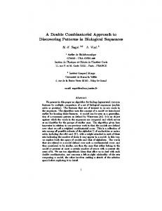
Fig. 1. Average grayscale images from adult subjects after a single iteration of translation correction (left) and after full affine alignment (right). The registration was performed using corresponding segmentations and the grayscale images are viewed here to visualize alignment. For the purpose of investigating the algorithm, 14 adult images were segmented using a previously published method and the segmentations (gray matter, white matter, cerebrospinal fluid) were registered using the proposed algorithm. In order to visualize the results, the transforms derived by aligning subject segmentations were applied to the associated grayscale MR images and the resulting images were normalized to a common mean and standard deviation and then summed. Figure 1 shows the results from this experiment. On the left is an initial alignment between subjects based on center of mass. On the right is the resulting segmentation. Despite gross initial misalignment, our algorithm identifies common structure in a typical anatomy estimate which is refined across iterations as the data becomes better aligned. In order to confirm that the metric maximum was properly found, each subject’s image was rotated from -10 degrees

to +10 degrees in one degree increments around the solution found during the group optimization procedure. This procedure was repeated for each axis and similarly for translations, along each axis, from -10 to +10 voxels. We confirmed that the algorithm properly converged to the optimum for each subject’s registration. One key feature of the described algorithm is the utility of the resulting typicality parameters. These statistics give feedback on how well subjects match, after alignment, and therefore how much residual variability remains. In order to demonstrate this, we created an atlas from ten fullterm infants and proceeded to register this pre-made atlas to a new cohort comprising 5 fullterm infants, 5 preterm infants, and one particularly sick, very preterm infant. We expected, based on previous research, that an affine transform model would properly account for the different size and shape of the preterms, compared to a fullterm atlas[3], but that the one outlier subject would show residual differences. Figure 2 shows an initial mean grayscale image demonstrating the several unaligned groups. Shown second is the same mean grayscale image, but with the gray matter atlas image overlaid in a starting configuration based on center of mass. The rightmost images are after alignment and show proper alignment of the subjects to one another and to the pre-computed atlas. Figure 3 shows a summary of the statistics computed by the atlas construction process. The L2 norm of the log of the affine component of the transform used to bring the subjects into alignment with the atlas is used as a measure of the magnitude of the alignment. As expected, aligning preterms to a fullterm atlas required more scaling than when aligning the fullterms to a fullterm atlas (left graph). Furthermore, the one outlier individual required the most scaling. We suspected that an affine alignment would successfully capture most of the differences between preterms and fullterms and this is illustrated in the rightmost graph. The trace mean of the typicality parameters gives a concise measurement of how well a subject matches the atlas after alignment. Both the preterms and fullterms are similar after alignment, but the outlier individual, due to severe structural differences, remains substantially different than the other two groups. 4. DISCUSSION AND CONCLUSION We have developed a novel method for the construction of a statistical atlas from segmentations. Our algorithm automatically determines how typical each subject is and identifies a common coordinate system. Construction of this coordinate system is influenced by each individual’s anatomy in a manner proportional to their typicality, and typicality statistics indicate how well each tissue class in each subject’s segmentation matches the derived atlas after alignment. We have demonstrated an implementation of this algorithm using a cohort of adult segmentations. Furthermore, we illustrated how the typicality parameters can be combined with measures of

219 Authorized licensed use limited to: Harvard University SEAS. Downloaded on September 15, 2009 at 16:02 from IEEE Xplore. Restrictions apply.

Fig. 2. Average grayscale brain images from eleven newborn infants (gray images) before (left) and after (right) registration. The color images show initial (left) and final (right) alignment with respect to the cortical gray matter channel from a precomputed full-term newborn atlas.

Fig. 3. Registration of very preterm (n=1), preterm (n=5), and fullterm (n=5) newborn infant brains to a newborn atlas as shown in Figure 2. The left graph shows that the children born earlier require more scaling to align to a fullterm atlas than fullterms. The rightmost graph shows that preterm and fullterm infants both appear similar after alignment with the atlas, however the one very early preterm (marked “outlier”) remains quite different. The chosen transform model is therefore able to capture the differences between preterms and fullterms, but not the outlier child. transform magnitude to describe how much subject variability is captured by the alignment and how much remains. We have used this scheme to differentiate healthy preterms, healthy fullterms, and one particularly affected preterm newborn infant, illustrating the utility of these measures. Future work will include investigation of different transform models and an extension to clustering of data into natural groups. 5. REFERENCES [1] Jean Talairach and Pierre Tournoux, Co-Planar Stereotaxic Atlas of the Human Brain, Thieme Medical Publishers, Inc., New York, 1988. [2] M Wilke, V J Schmithorst, and S K Holland, “Normative pediatric brain data for spatial normalization and segmentation differs from standard adult data.,” Magn Reson Med, vol. 50, no. 4, pp. 749–757, 2003. [3] AU Mewes, L Z¨ollei, PS Huppi, H Als, GB McAnulty, TE Inder, WM Wells, and SK Warfield, “Displacement of brain regions in

preterm infants with non-synostotic dolichocephaly investigated by MRI.,” Neuroimage, 2007. [4] Alexandre Guimond, Jean Meunier, and Jean-Philippe Thirion, “Average brain models: a convergence study,” Comput. Vis. Image Underst., vol. 77, no. 9, pp. 192–210, 2000. [5] Daniel Rueckert, Alejandro F. Frangi, and Julia A. Schnabel, “Automatic construction of 3D statistical deformation models of the brain using non-rigid registration.,” IEEE Trans. Med. Imaging, vol. 22, no. 8, pp. 1014–1025, 2003. [6] M. S. De Craene, B. Macq, F. Marques, P. Salembier, and S. K. Warfield, “Unbiased group-wise alignment by iterative central tendency estimations,” Math. Modelling of Natural Phenomena, vol. 3, no. 6, pp. 2–32, 2008. [7] A. Dempster, N. Laird, and D. Rubin, “Maximum-likelihood from incomplete data via the EM algorithm,” J. Royal Statistical Soc. Ser. B, vol. 39, pp. 34–37, 1977.

220 Authorized licensed use limited to: Harvard University SEAS. Downloaded on September 15, 2009 at 16:02 from IEEE Xplore. Restrictions apply.