The Randomized Sample Tree: A Data Structure for Interactive Walkthroughs in Externally Stored Virtual Environments Jan Klein∗ Jens Krokowski∗ Matthias Fischer∗ Michael Wand† Rolf Wanka∗ Friedhelm Meyer auf der Heide∗ ∗ University
of Paderborn
† University
of T¨ubingen
May 31, 2005
Abstract We present a new data structure for rendering highly complex virtual environments of arbitrary topology. The special feature of our approach is that it allows an interactive navigation in very large scenes (30 GB/400 million polygons in our benchmark scenes) that cannot be stored in main memory, but only on a local or remote hard disk. Furthermore, it allows interactive rendering of substantially more complex scenes by instantiating objects. The sampling process is done in the preprocessing. There, the polygons are randomly distributed in our hierarchical data structure, the randomized sample tree. This tree only uses space that is linear in the number of polygons. In order to produce an approximate image of the scene, the tree is traversed and polygons stored in the visited nodes are rendered. During the interactive walkthrough, parts of the sample tree are loaded from local or remote hard disk. We implemented our algorithm in a prototypical walkthrough system. Analysis and experiments show that the quality of our images is comparable to images computed by the conventional z-buffer algorithm regardless of the scene topology.
1
Introduction
Despite the use of advanced graphics hardware, real-time navigation in highly complex virtual environments is still a fundamental problem in computer graphics because the demands on image quality and details increase exceptionally fast. There are several sophisticated algorithms to ∗ Faculty
of Computer Science, Electrical Engineering & Mathematics and Heinz Nixdorf Institute, University of Paderborn, 33095 Paderborn, Germany. Email:{janklein, kroko, mafi, wanka, fmadh}@uni-paderborn.de † University of T¨ ubingen, WSI/GRIS, Sand 14, 72076 T¨ubingen, Germany. Email:
[email protected]
1
overcome this problem but scenes of arbitrary topology that cannot be stored in main memory are still very difficult to handle. A very interesting application field for our proposed approach is navigation in virtual environments consisting of many different detailed objects, e.g., of CAD data that cannot all be stored in main memory but only on hard disk. E. g., such a navigation would be very useful in the area of plant layout. On the one hand, one wants to get an overview of all models by viewing from far away, and on the other hand one wants to examine single objects very closely. Therefore, it is desirable to store only the polygons with their appropriate attributes (e.g., textures, colors) and not to produce additional data as, e. g., additional textures for image based rendering or precomputed LODs: Then, the viewer can operate with the original data and images of high quality can be rendered independently of the scene topology and the camera position. Furthermore, the polygons of such highly complex scenes require a lot of hard disk space so that the additional data could exceed the available capacities. For these requirements, an appropriate data structure – the randomized sample tree – has to be employed with a memory consumption that is linear in the number of polygons. Our work is motivated by the following two main requirements: 1. Interactive rendering of complex scenes: We want to achieve interactive rendering of complex static scenes in output-sensitive time, i.e., the rendering time should be sublinear in the number of polygons. To achieve this, we reduce the scene complexity by only rendering samples of polygons that approximate the scene. Our measurements show that the rendered samples of polygons are small enough to generate interactive frame rates and large enough to generate images of a good quality. We assume that the samples of polygons needed for the computation of one frame can be stored in main memory. In practice, this is no real restriction because the samples are very small even for our most complex scenes. 2. Complex scenes stored on hard disk: We focus on navigation through highly complex scenes that cannot be completely stored in main memory. The number of polygons in a scene should only be restricted by the size of the hard disk. This is of special interest for scenes consisting of many different types of models for which instantiation schemes [35] cannot be used. Generally, storing the data causes expensive hard disk accesses which have to be minimized in order to achieve interactive rendering. We solve this as follows: The samples are computed in the preprocessing and are stored in a sample tree on hard disk. During navigation, needed nodes and their polygon data must be loaded. To exploit temporal coherence, we use a caching mechanism so that only very few nodes have to be loaded from one frame to the next (we assume that the viewpoint does not move over great distances within a short period of time). Furthermore, the samples that are stored in the nodes are small so that there is little polygon data to load from hard disk for each image. In the following, we give a short overview of further aspects and features of our algorithm. Network-based rendering: We implemented our algorithm in a client-server network: The sample tree is stored on a remote server connected to the client via TCP/IP. During a walkthrough the client loads parts of the polygon data from the remote hard disk into its main memory and sends them to its graphics subsystem. In Section 7, we show that for networks with a high bandwidth, good frame rates can be achieved. This client-server concept is similar to the concept of a scene manager used in [28]. Arbitrary scene topology: Our proposed approach requires neither a special type of a vir2
q u a d tre e c e ll
s a m p le tre e
p o ly g o n
Figure 1: Sample tree for a 2D scene with a quadtree. tual environment nor a special scene topology. In our evaluation, we use different kind of scenes to demonstrate the flexibility: our algorithm achieves interactive frame rates in landscape scenes with millions of coarsely modelled objects in combination with highly detailed scene parts. Furthermore, it can be used for the visualization of thousands of highly detailed objects, like the well-known happy buddha. Thereby, close views of single objects cause no problems. Also, the quality of the images computed by our algorithm is independent of the scene topology and the camera position. Holes or disconnectivities in the models cause no problems. The input for our algorithm is the polygonal description of the virtual environment, e.g., triangles, normals, material colors. Until now, our system does not provide textured objects but it should be easily possible to provide this feature. A typical scene for our approach may consist of many different models (e.g., landscapes with trees, buildings and cars). Efficiency: We need neither complicated level-of-detail computation of the polygons nor memory-expensive replacement by textures or prefiltered points. The space for storing our sample tree is only linear in the number of polygons: Every polygon is stored exactly once in the tree and in practice – our measurements confirm this –, the number of nodes is at most the number of all n polygons because every node contains at least one polygon. Therefore, storing the tree costs only O(n) space and the constant is very small, e. g., between 1.04 and 1.30 for our test scenes. This is a great advantage because our scenes are highly complex and have to be stored on hard disk. The test results with our prototypical walkthrough system show that our approach works with scenes consisting of more than 400 million polygons, whereby every polygon is separately stored on hard disk. Our results show that an approximate image with 640 × 480 pixels can be computed within 326 msec if the sample tree is stored on a remote hard disk.
2
Outline of our Approach
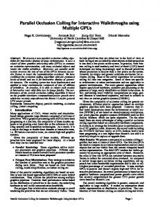
The sample tree: Our rendering algorithm uses a so-called sample tree which is an octree-like data structure for the spatial organization [4] of the polygons. In every node a sample of polygons is stored that approximates the corresponding cell if the viewpoint is far away from the cell. An exact definition of far away is given in Section 4. The leaf nodes store all polygons that were not chosen for the samples in any ancestor nodes. Figure 1 demonstrates the idea of our sample tree. In order to pick a sample for the root node of the sample tree, our tree construction algorithm chooses polygons from the whole scene 3
Figure 2: The Happy Buddha rendered by our approach (middle) and the magnifications of the face in object space (left) and image space (right). depending on their areas and stores them in the root node. These polygons are marked in yellow in our example. They give a good approximation of the scene if the viewpoint is far away from the cell; in this case the viewpoint would lie far outside of the whole scene. In order to get a sample for the upper left quadtree cell, we randomly choose polygons from the corresponding cell, the probabilities depending on their areas (we do not consider polygons that are already stored in the root node). The chosen polygons, marked in red, lying in the cell together with the yellow polygons stored in the ancestor node give a good approximation of the upper left quadtree cell if the viewpoint is far away from it. Rendering of the scene: In order to produce an image of the scene, the sample tree is traversed by a depth-first search and all polygons lying in visited nodes are rendered. The traversal stops at a node u if the corresponding cell is far away from the viewpoint. Then the distance from the viewpoint to the cell of u is so large that the sample stored in u gives a good approximation of the cell. If the traversal stops at a leaf node v, all polygons lying in the corresponding cell are rendered. If, in this case, we rendered only a sample of polygons, the approximation would result in low image quality because the viewpoint is close to the cell. This kind of traversal is well-known in the context of LOD systems (e. g., see [21]). The following two examples illustrate the effect exploited by our method: The middle images of Figures 2 and 15 are rendered by our sampling technique as described above. We have frozen the sample sets and magnified parts of the scenes in object space. The middle image of Figure 2 shows the Happy Buddha[7] and the left image illustrates the polygons of the sample set that are rendered for the face. As one can see, the surface of the sampled polygons is incomplete in object space but these polygons give a good approximation for the viewpoint of the middle image. The selected polygons are sufficient to create a contiguous image of Happy Buddha’s face as demonstrated on the right of Figure 2 which is a magnification in image space. In Figure 15, we zoomed into two parts of an image of a landscape scene rendered by our 4
se rv e r
T C P /IP
s a m p le tre e
s a m p le tre e
H D D
n o d e m a n a g e r
re n d e rin g w o rk s ta tio n (c lie n t)
n o d e id n o d e
re n d e rin g a lg o rith m
m e m o ry
p o ly g o n s
g ra p h ic s s u b s y s te m
Figure 3: Walkthrough system: client and server connected via TCP/IP, the polygon data are stored on hard disk. method. One can see that the objects are incomplete and that only samples of polygons are rendered. Below the two zoomed pictures, the corresponding complete parts of the original scene rendered by the z-buffer algorithm are presented for comparison. Observe that for nodes lying in the part closer to the viewpoint the tree traversal is aborted later than for nodes in the part far away. One can see, e. g., that more polygons of a house are rendered in the front part than for houses lying in the other part. Client-server walkthrough system: For highly complex scenes, if the scene does not fit into main memory the sample tree can only be stored on a local or remote hard disk. The walkthrough system consists of a rendering workstation (client) and a node manager (server) that handles the sample tree stored on its local disk (see Figure 3). The rendering algorithm (client) traverses the sample tree during the walkthrough and sends the polygons stored in the visited nodes to the graphics subsystem. If a node of the sample tree is not available in main memory, the rendering workstation loads it via TCP/IP from the node manager.
3
Related Work
Several approaches have been proposed for accelerating the rendering of complex 3D scenes. In the following, we summarize related work in the area of point sampling, out-of-core rendering and network-based walkthroughs. Furthermore, we look at the possibility of adapting occlusion culling to our approach. Point sample rendering: Our rendering technique has the most in common with point sample rendering. Like these methods, we draw samples of the scene objects and render them in order to reduce time-expensive rendering of all polygons. In the 1970’s and 1980’s several researchers had already proposed to use points as display primitives [2, 17] because their rendering and rasterization is simple and cheap. Additionally, point sample rendering is independent of the scene topology in contrast to mesh-based multiresolution models. Recently, research has focused again on point sampling. Grossman and Dally [14] use points both as rendering and as modelling primitives. QSplat [25] and Surfels [24] apply prefiltering methods to convert graphics primitives into a uniform point representation. The points are selected from a LOD-like representation according to their screen projection. This results in a low rendering time and high image quality. 5
QSplat [25] works best for large, dense models containing relatively regular, uniformly spaced points. The problems are sharp corners and subtle curves. A further problem occurs if objects are viewed very closely and if points are projected to more than one pixel, it results in blocky images. A solution to overcome this problem is the interpolation between adjacent points which sometimes results in artifacts [24]. A further solution for the problem of close views is given by [1, 30, 34], who use locally adapted sample densities for the rendering of complex geometry. Chen and Nguyen [3] use triangles and points for the rendering of large mesh models with the ability of close views. In contrast, our approach generally uses polygons for rendering. Points or splats can additionally be used in order to get coarser approximations and to improve the rendering times. There are some advantages of mainly using polygons: First of all we produce no additional data like, e.g., textures so that we have a memory consumption that is linear in the number of polygons. This cannot always be fulfilled by point-based methods. Moreover, the viewer can operate with the original polygon data which could be useful for some applications, for example, in the area of plant layout. Another point is that our method is able to render images of high quality independent of the scene topology and the camera position and therefore we have no problems with close views. Wand et al. [34] proposed a technique for randomized point sampling. For each frame they have to choose new sample points by using hierarchical concatenated distribution lists. In combination with a caching mechanism they are able to render complex scenes at interactive frame rates. But their technique can only handle scenes which can be completely stored in main memory. Furthermore, their method produces images of bad quality if some polygons are parallel and lie close to each other. Our proposed approach overcomes these two drawbacks: In Section 4 we prove that images of good quality are produced by our algorithm whereby no assumption about the position of the polygons is made. The other problem – the limitation to main memory – is solved by our sample tree: We have developed a sampling technique that can be done in the preprocessing whereby the polygons can easily be stored on hard disk. Because we do not use any distribution lists like Wand et al. [34], where expensive dynamic updates have to be done for each frame, our randomized sampling method saves enough time that can be used for the data transfer from hard disk. So in contrast to Wand et al. we are able to handle scenes consisting of many different models that cannot all be stored in main memory but only on hard disk. Note that although we sample only once in the preprocessing instead for each frame we can prove that our images are always of good quality. Out-of-core rendering: Recently, Lindstrom and Pascucci [18] present a framework for out-of-core visualization of terrain surfaces. Their results show that this approach works well with large terrain meshes consisting of about 5 GB polygon data but it does not really fit to scenes of arbitrary topology as our approach does. The system presented by Sobierajski Avila and Schroeder [29] allows an interactive navigation through large polygonal environments produced by CAD systems. Thereby, they combine view frustum culling and LOD modelling. In comparison, our method does not use a limited number of different LOD representations but every polygon is only stored once in the sample tree. Furthermore, our approach adjusts the approximation quality within a single object during the navigation. So we can achieve a smooth navigation without the effect of toggling between different LOD representations. 6
Wald et al. [32, 33] propose distributed ray tracing as a technique for interactive rendering. In [32] it is shown that they are able to generate very high quality images of scenes consisting of 50 million polygons stored on hard disk. They achieve interactive frame rates by using seven dual Pentium PCs. It is obvious that ray tracing produces images of higher quality than conventional rendering methods but generally ray tracing has a worse performance than rasterization algorithms. Network-based walkthroughs: Transmitting 3D data across a network has become an interesting field of research. As our approach allows not only rendering of highly complex scenes stored on a local hard disk but also stored on a remote hard disk, we survey shortly related work in the area of network-based rendering. In the context of occlusion-culling, the PVS approach presented by Teller and S´equin [31] is suitable for a client-server system. Thereby, the server computes the PVS (Potentially Visible Sets) and sends them to the client to avoid the transmission of invisible geometry [10, 11]. In order to use the network capacity consistently despite of sharply changing viewpoints, Cohen-Or and Zadicario [6] propose a prefetching of an ε-neighborhood to ensure that off-screen objects are loaded into memory. Mann and Cohen-Or [22] present another system of collaborating client and server. They assume that web-based virtual environments are dominated by huge amounts of texture data which are stored on the server, while the models are locally available at the client. The network requirements are reduced by sending only the difference image needed for the current view. Schmalstieg and Gervautz [27] employ the notion of “Area Of Interest” (AOI) in the context of multi-user distributed virtual environments where AOI is a circular area around the viewpoint. Only the objects in this area are sent from the server and stored in main memory of the client in order to reduce the network transmission. In contrast to their approach, we also render objects that are far-off so that we do not have the effect of objects popping into an image. Streaming transmission of data sets has become interesting because of growing network speed. Sophisticated algorithms transmit low-resolution data first, so the user sees a coarse approximation and can interact with the scene. Then, a progressive stream of high-resolution data improves the quality. There are some polygon-based approaches that are suitable for this kind of multi-resolution rendering: Hoppe’s progressive mesh approach [16] represents a model by a base mesh and refinements to this mesh. The mesh correction can take place by vertex split operations [16] or by wavelet encoded operations [8]. Rusinkiewicz and Levoy [26] employ a multi-resolution point rendering system for the streaming of large scenes. A splat-based bounding box hierarchy is used for a view-dependent progressive transmission of data across a network of limited bandwidth.
7
Occlusion culling: In the last few years many occlusion culling algorithms have been developed, see the survey of Cohen-Or et al. [5] for a detailed overview. We have not focused on any occlusion culling yet, because point sample rendering and occlusion culling are two orthogonal problems. We only perform view frustum culling and backface culling. The running time of our approach depends linearly on the projected area a of s sampled polygons, including hidden polygons. Since we use the z-buffer algorithms for rendering the sampled polygons, the running time is O(s + a) [15]. Thus, our algorithm becomes inefficient if there are many polygons near to the viewer because these polygons have a great projected area. But we think, our sample tree fits well to known occlusion culling algorithms [9, 13] because the polygons are managed in a spatial and hierarchical way that can be used for the visibility tests.
4
The Randomized Sample Tree
In this section, we describe the idea and the structure of the sample tree and how an image of the scene is rendered. Furthermore, we show how the samples of polygons have to be chosen so that, with arbitrarily high probability, a correct image is produced. In the last two subsections, we describe extensions of our algorithm to improve the image quality and to accelerate the rendering time. In order to explain the main idea of our sample tree, we need the notion of correct image. Correct image: A part of an image with size ≤ 1 pixel is called correct if at least one visible polygon r from this part is rendered. The whole image is correct if all of its parts are correct. A discussion of this definition follows at the end of section 4.3. A correct image may still show aliasing and noise artifacts. Wand et al. [34] deal with these problems by averaging over several independent renderings resulting in a slow rendering time. This technique is not possible in our case as we employ fixed, precomputed sample sets. However, the same effect can be achieved by supersampling, i.e., rendering the image at a higher resolution and sampling density and then downsampling the image.
4.1
The Data Structure
In the following, we explain the hierarchical structure of our sample tree, which corresponds to a modified octree, and the insertion of the polygons into its nodes. The octree cell of a node u is called B(u). Let A(r) denote the area of the polygon r. Furthermore, let P(u) denote all polygons of a scene lying in B(u) and let A(P(u)) denote the sum of all areas of polygons from P(u), i.e., A(P(u)) = ∑r∈P(u) A(r). The idea of our sample tree is that in every inner node u, a sample of the polygons P(u) is stored. We store sufficiently many polygons in a node u, so that these polygons, together with the polygons stored in the ancestor nodes of u, approximate well P(u) if the viewpoint is far away from B(u). Approximate well means that the projection of the polygons produces a correct part of the image with high probability p. The probability p depends on the sample size mu , that, in turn, depends on A(P(u)). For details, see Section 4.3. To pick a sample stored in a node u we look at all polygons P(u) and add a polygon r to the sample set with a probability proportional to its area, i.e., with probability A(r)/A(P(u)), 8
because on average larger polygons contribute more to an image than smaller ones. Far away means that the projected bounding box of B(u) is at most one pixel. So, in every inner node u, a sample of polygons is stored that approximates P(u). A leaf node v contains all polygons from P(v) except those polygons that are already stored in any direct or indirect ancestor node of v. Analogously, a polygon is not stored in any inner node u if it is already stored in an ancestor node of u. That means that every polygon is stored exactly once in the tree. Figure 4 presents the algorithm that computes a sample tree. Before starting it, an octree has to be constructed where polygons are inserted in leaf nodes or recursively in the ancestor nodes if they do not fit completely into a bounding sphere of a leaf node. The algorithm has to be started with the root node of the octree. The sample size mu can be computed from Theorem 1 (Section 4.3). One has to consider that many other very small polygons would be inserted into high-level nodes (nodes near to the root node), if they lie on edges of any octree cells. As a consequence, these polygons would be rendered for nearly every image. To avoid this behavior, the algorithm can easily be modified: Instead of choosing polygons from P(u) we choose them from all polygons lying in the bounding sphere of B(u). createSample ( node u ) if u is not a leaf node for every child d of u do createSample ( d ) M = 0/ compute mu for i = 1 to mu do choose polygon r from P(u) with probability A(r)/A(P(u)) store the chosen polygon in set M remove the polygon from any child node of u store all polygons from M in node u Figure 4: The algorithm constructs a sample tree in bottom-up manner. Its input is the root of a precomputed octree.
4.2
Rendering an Image
In order to render an image, the sample tree is traversed by a depth-first search and all polygons stored in visited nodes are rendered. The traversal is stopped at a node u if the projected bounding box of B(u) is at most one pixel. Then the polygons stored in u are rendered and produce a correct part of the image with arbitrarily high probability that depends on the sample size mu . If the traversal is not aborted, the search ends at a leaf node v. Consequently, all polygons of the scene lying in B(v) are rendered.
9
Note that all polygons stored in visited nodes have to be rendered. It is not sufficient to render only polygons stored in nodes where the traversal stops since P(u) is only approximated by the polygons in u and the ancestor nodes together. Our method renders all polygons having a projected area of more than one pixel because the traversal stops at a node u if its projection is at most one pixel, and polygons that do not fit completely into the bounding sphere of B(u) are stored in ancestor nodes.
4.3
Sample Size
In this section, we explain how many polygons have to be chosen for each sample. Furthermore, we prove that enough polygons are stored in every node to produce correct images with arbitrarily high probability. We choose polygons randomly with a probability proportional to their areas. That means we add a polygon r to the sample with probability A(r)/A(P(u)) because on average larger polygons contribute more to an image than smaller ones. It is obvious that the larger the sum of all polygon areas in a cell is, the larger the sample should be in order to compute a correct image. It is important to properly estimate the size of the sample, as too many polygons result in slow rendering and too few polygons result in a low image quality. Therefore, Theorem 1 shows how many polygons have to be stored in a node u. Theorem 1 (Sample size): Let A(P(u)) denote the sum of all areas of polygons from P(u), and let A(B(u)) denote the area of one side face of the bounding box of B(u). The factor qu is defined as qu = dA(P(u))/A(B(u))e. Let c be an arbitrary constant. If mu = qu · ln qu + c · qu independent drawings from P(u) are done and the chosen polygons are stored in the node u, −c then with probability p ≈ e−e their projection gives a correct part in the image for an arbitrary viewpoint if the projection of B(u) is at most one pixel and if the area of the projected polygons from P(u) shows no holes from any viewpoint. Proof: We have to guarantee with probability p that from an arbitrary viewpoint, there is always a visible polygon in the sample stored in the node u. Then, as the projection of B(u) is at most one pixel and as we render a visible polygon with probability p, the corresponding part of the image is correct (with probability p). Note that the following described operations neither have to be done during the preprocessing phase nor during the navigation. They are only used for proving the theorem. Let Vu denote the viewing ray through the center of B(u). We consider an arbitrary, but fixed viewpoint in the scene so that the projection of B(u) is at most one pixel. Let fmax be the maximum area of a surface that is orthogonal to the viewing ray Vu and that completely lies in B(u) (see Figure 5 (a)). The minimal sum of the area of all visible polygons from P(u) amounts to fmax because we assume that from any viewpoint the area of the projected polygons from B(u) shows no holes. If some visible polygons are not orthogonal to the viewing ray Vu , the area of all visible polygons or parts of polygons will be greater than fmax . For the sake of argument, let us partition the polygons from P(u) into qeu groups so that all polygons of each group (except the last one) have a total area of fmax . For this, polygons might have to be subdivided and to be put into two groups. qeu can be computed as qeu = dA(P(u))/ fmax e.
10
All visible polygons or parts of visible polygons lying in B(u) are put into one group. They fill at least one group because they have a minimum area of fmax as described above. Now the question is how many polygons mu have to be chosen in such a way that with probability p from each group at least one polygon is taken. By choosing at least one polygon from each group, you would have chosen at least one polygon from the group of the visible ones. Consequently, if mu polygons are stored in u, a visible polygon from P(u) is between these mu polygons, seen from an arbitrary but fixed viewpoint. When all mu polygons are rendered, the visible polygon is rendered too. As B(u) is at most one pixel, the corresponding part of the image is correct. The question raised above can be answered with the help of the reduction to a simple urn model: Given a bins, how many balls have to be thrown randomly and independently with the same probability into the bins so that every bin gets at least one ball? The number a of the bins corresponds to the number qeu of the groups and the number of balls corresponds to the number of necessary drawings of polygons. Let X denote the number of drawings required to put at least one ball into each bin. It is well known (e.g., see [23, p. 57f]) that the expectation value of X is qeu · Hqeu where Hqeu is the qeu -th harmonic number. Let c be an arbitrary constant. The qeu -th harmonic number is about ln qeu ± 1 which is asymptotically sharp, and so c · qeu additional balls are enough to fill each bin with probability p which depends on c. Consequently, mu = qeu · ln qeu + c · qeu polygons from P(u) have to be chosen and stored in u. To compute the dependence of p on c, we refer to the proof in the textbook of Motwani and Raghavan [23, p. 61ff]. They showed that the probability p of X ≤ mu is equal to −c p = e−e for a sufficient large number of bins. Until now we considered an arbitrary, but fixed viewpoint so that the projection of B(u) is at most one pixel. The size of the sample depends on qeu and qeu depends on the viewpoint: If the viewpoint is chosen so that fmax is minimal, qeu — the ratio of A(P(u)) and fmax — is maximal. It is obvious that the minimal size of fmax corresponds to the area of a side face s of the bounding box of B(u). Then the viewpoint is chosen so that the viewing ray Vu is orthogonal to the side face s (see Figure 5 (b)). All other viewpoints result in a greater area fmax . So qeu is maximal and equal to qu if fmax is equal to A(B(u)). Therefore, the maximal number of polygons which have to be chosen from P(u) and stored in the node u can be estimated by mu = qu · ln qu + c · qu . Corollary 1 (Correctness of an image): Let c be an arbitrary constant and let j denote the number of nodes where the traversal did not continue to child nodes. The sample size in every −c node u is chosen so that with probability p ≈ e−e the polygons of the sample produce a correct part of the image. Then the probability of a correct image is p j . Proof: We produce a correct image of the scene with probability p j because for all j nodes where the traversal stops, the corresponding area of the image is correct with arbitrarily high probability p. All other areas in the image are correct anyway because all polygons in these areas are rendered. In practice, it is no problem to choose a sample size so that p is always greater than 1 − 10−6 . Therefore, c ≈ − ln 10−6 ≈ 13.8 has to be set. If the factor j is about 104 , this is a realistic value in practice, and if we store mu = qu · ln qu + 13.8 · qu polygons in every node u, we generate a correct image with probability p j > 0.99.
11
B(u)
Vu
B(u)
fmax
Vu
fmax
(a)
(b)
Figure 5: (a) The grey surface is orthogonal to the viewing ray Vu . This surface with an area of fmax lies completely in B(u). (b) If the viewing ray Vu is orthogonal to a side face of B(u) then fmax will be minimal.
4.4
Discussion of the Definition of a Correct Image
In the context of model approximation the discussion about correct images and image error metrics occupies computer graphics already very long [15]. Many simplification methods use an error metric to regulate the quality of the simplification [19] or to preserve the similarity of appearance [12]. A lot of useful suggestions exist, but until now [20] there is not any unambiguous universal solution for all applications. With our definition of a correct image we want to show the forte and weakness of our approach. The aim of our algorithm is the fast rendering of highly complex scenes with an image quality, that is comparable with that of the z-buffer algorithm. Comparable image quality means, that we attempt to minimize the number of pixels, which have another color, as the pixels of an image of the z-buffer algorithm. In the following we show why our rendered images cannot be completely identical to those of the z-buffer algorithm. p o ly g o n s w ith s a m e z v a lu e x y z
b
a
o n e P ix e l
B (u )
v ie w in g r a y z
c
c
y
x
b
a
o n e P ix e l v ie w in g r a y
Figure 6: The Figure shows the space behind a pixel (frustum), the short lines are polygons. There are the visible polygons a, b, c and the invisible polygons x, y, z. Polygon a is nearest and z is farthest w.r.t. the viewpoint. First of all we look at a typical error of the z-buffer algorithm, which arises due to the limited accuracy of the z value. The Figure 6 (left) shows an example. There are the visible polygons 12
a, b, c and the invisible polygons x, y, z which are masked by the visible polygons. We assume that the polygons a, b, x, and y have the same minimum z value, therefore the pixel gets the color of one of these four polygons. Which one of the four polygons affects the color depends on the implementation of the graphics system. If the pixel gets the color of the invisible polygons x or y we get a visibility error (z-buffer error). In the following we call such kind of invisible polygon a bad polygon. Figure 6 (right) shows an example of a situation of our rendering algorithm. Let the traversing of the sample tree be stopped at the cell B(u). Furthermore, we assume, that all polygons a, b, c, x, y, and z have different z values. The following error can occur: our definition guarantees that at least one visible polygon of the cell is selected (w.h.p.), but we cannot guarantee, that this is the nearest polygon of the cell B(u). If the random sample set consists of the polygons b and x, the pixel gets the color of the invisible polygon x and causes a visibility error. In this situation polygon x is a bad polygon. It remains the question how strong this error can take effect on the image quality. The example of Figure 6 (left) shows that sometimes the pixel gets the color of an invisible polygon (bad polygon, z-buffer error). We ask now for the position of the bad polygons in the scene and their distance to visible polygons. In case of the z-buffer error, the bad polygons are always near to the visible polygons. In case of our rendering algorithm the situation is similar: The bad polygons must be contained in the cell B(u), or their neighboring cells. Because we guarantee (w.h.p.) that at least one visible polygon is selected from the cell B(u), this polygon is nearer than all polygons that are behind the cell, e.g., in Figure 6 (right) the polygon z can never be a bad polygon and cause an error. A discussion of the differences between the z-buffer and our approach concerning the image quality in practice is given in section 7.1.
4.5
Precomputation of Color Values
To summarize, one can say our method renders all polygons having a projected area of more than one pixel and renders only a representative sample of polygons for smaller ones. The traversal stops at a node u if its projected cell B(u) is at most one pixel. All polygons in such a node u are projected onto an area of the image with a size of at most one pixel and cover only parts of a small neighborhood of pixels. Which color value is attached to the pixel eventually depends on the depth of the z-buffer, the sequence of the projected polygons and the graphics library that is used. In order to improve this procedure with the aim to get a better color value for the pixel, a color value that is representative for all sampled polygons stored in a node u can be determined. This color value is rendered with the size of one pixel instead of the corresponding polygons, if the projected bounding box of B(u) is at most one pixel. In our implementation the color value is determined as the median of all sampled polygon colors depending on the polygon areas. It is also conceivable to calculate a better color value by using Gaussian filters and considering adjacent color values.
13
4.6
Far-Off-Splatting
In the context of point sample algorithms the notion of splatting has become popular in the last few years. Instead of rendering points or single pixels many approaches render splats in order to reduce rendering time and to guarantee that the images show no holes. Based on this idea we developed the far-off-splatting. Thereby, objects far-off are mainly represented by splats and only the larger polygons are rendered for these objects. For objects near to the viewer it is the other way round: Generally, polygons are used for drawing them and splats are only used sparsely so that the image quality of these objects is good. With this technique the rendering times can be improved while the images are of good quality. Specifically the far-off-splatting works as follows: Instead of traversing the tree until the projected bounding box of a node is at most one pixel, the traversal can be stopped earlier at a node u, if its projected bounding box is at most i2 pixels, i ∈ {1, 2, 3, . . .}. For such a node u, a color value computed in the preprocessing is rendered as a splat of size i2 pixels instead of the polygons stored in u. We denote i as the splat size. Thereby, we ensure that there are no holes in the rendered images. Note that the projection of bounding boxes near to the viewer is mostly larger than i2 pixels (for small i) so that the corresponding polygons are rendered and a high image quality can be achieved.
5
External Construction of the Sample Tree
If the scenes are highly complex and cannot be completely stored in main memory, the sample tree cannot be constructed in an easy top-down manner. The problem is that for every node u one has to draw a polygon mu times from all polygons P(u). This cannot be done within an acceptable amount of time in the preprocessing phase because only a small part of polygons can be stored in main memory. Many hard disk accesses would be necessary. To overcome this problem we construct the sample tree in a bottom-up manner that differs a little from the algorithm described in Section 4.1 (see Figure 4). For this purpose, we have to construct an octree from which afterwards our sample tree is built and stored on hard disk. The octree has to be precomputed because we have to know which polygons lie in each leaf node of the sample tree at the beginning of its construction.
5.1
Octree Construction for Large Scenes
One problem to be solved is that one cannot store every node of the octree or of the sample tree in a single file. During the construction, as well as during the walkthrough, too many files would have to be opened and closed which would result in a long preprocessing time or in a high response time of the node server. Another problem to overcome is how to store all nodes with their polygon data. This cannot be done in a single file because its size is restricted by most operating systems. Furthermore, it is important to store nodes of neighboring cells in a single file because often these nodes are requested immediately one after another. Because of these problems, an octree is first constructed in two steps: In the first step, the
14
... |
node i
node i + 1
...
... }|
{z node data
polygonal data of node i {z polygonal data
... }
Figure 7: File layout. structure of the octree is determined (determine structure) and in the second step the polygons are stored in the file of the corresponding node (storing polygons). Determine structure: In this step, the structure of the octree of a fixed maximum depth d is built up. For every node, the number of polygons lying in the corresponding octree cell is counted. The final depth – by which it can be guaranteed that every leaf node does not store more than a fixed number of polygons – cannot be determined in advance because of the unknown spatial distribution of the polygons. So, we estimate the maximum depth d for which the structure will fit in main memory. During the construction d can automatically be decremented and the calculated structure can be adjusted if the required size of main memory is too big. After the hierarchy is completely constructed, each node gets a unique identifier. The nodes are enumerated by a breadth-first search and especially child nodes of one node get consecutive identifiers. Then the nodes are saved on the hard disk and storage is reserved for the counted polygons. If necessary, the data is split into more than one file if the maximum size of the file is reached. Figure 7 describes the layout of those files: A file consists of two blocks. The first one contains the node data with a fixed size for each node and the second block stores the polygonal data that can be of variable length for each node. The node data consists of the center and the size of the node, the identifier for the child nodes, the number of polygons and an offset to the polygonal data of the node. So, the position of the node data can easily be calculated from the value of the identifier and the time for accessing the data of one node with p polygons is O(p) or O(log f + p) if the octree is distributed to f files. Storing polygons: In the second step of the octree construction the polygons are stored in the file of the corresponding node. After this construction, leaf nodes are subdivided into subnodes if they contain more than a fixed number of polygons. Until now, we do neither any geometric compression nor any quantification like Rusinkiewicz and Levoy [26] do.
5.2
Sample Tree Construction
The octree described in the previous section can now be used to build our sample tree. We take the spatial subdivision of the octree for our sample tree. Now we have to distribute the polygons to the tree so that each node gives a good approximation. Note that the leaves of the octree already meet the property of a sample tree node: the polygons of a leaf node v approximate well P(v).
15
With this condition we build up our sample tree in a bottom-up manner. Given a node u which child nodes fulfill the sample tree property, we draw polygons from the direct child nodes, store them in u and delete them from the corresponding child nodes. It is important to draw the sample for u only from its direct child nodes instead of drawing it from all nodes of the subtree rooted by u. Therefore, the locality of data can be exploited and the runtime can dramatically be reduced, because as few polygons as possible are loaded from hard disk into main memory. As a consequence, we reduce expensive hard disk accesses and can build up the sample tree in an acceptable preprocessing time. This construction has the effect that polygons stored in the leaf nodes of the octree are shifted up successively.
6
Navigation in Externally Stored Scenes
To allow an interactive navigation in scenes stored on hard disk, the following requirements have to be considered: 1. To compute a new image, only a few nodes should be loaded. 2. Loading a node may take only very short time. An appropriate algorithm is described in this section. Thereby, we assume that the viewer moves only slightly between the computation of two successive frames. Also, we assume that the polygon samples needed for the computation of one frame can be stored in main memory. In practice, this is not a restriction because the samples are very small even for our most complex scenes.
6.1
Client-Server Model
In order to store scenes on hard disk and to load data during navigation, we have implemented a client-server structure (see Figure 3). The sample tree is stored on the hard disk of the server and is managed by the node manager. The client is connected to the server via TCP/IP and serves as a rendering workstation. Server and client can either be started on a single computer to store the scenes on local hard disk, or on different computers to store the scenes remotely. The traversal of the sample tree and the rendering of polygons are executed on the client. At the beginning, there is no sample tree on the client so that the client sends a request to our node manager with the unique node identifier of the root node. The received root node is stored in main memory. While the traversal has not stopped at a node u, and the required child node is not stored in main memory, the client sends requests to the server and stores the received nodes in memory. Of course, one cannot manage all nodes in main memory which are received during the walkthrough. For this, we developed a caching mechanism which removes nodes in main memory but keeps nodes that are needed for the next frames.
6.2
Caching and Deleting Nodes
In the previous section, we described the loading of nodes from hard disk. While moving through the scene, parts of it can be coarser approximated and the nodes of the finer approximation can
16
be deleted. To avoid deleting and loading the same nodes within a very short time, we use our caching strategy to keep some nodes in main memory. Our caching is simple but very efficient: If the traversal stops at a node u stored in the kth level of the sample tree, all child nodes of the next j levels are kept in main memory. j is arbitrary but fixed and measurements show that j ∈ {1, 2} provides the best results. All nodes of the next levels having a depth of more than k + j are deleted from memory. This method can be improved by implementing the data transfer of the nodes via TCP/IP and the rendering and the traversal in the sample tree to be asynchronous. That means if a request is sent to the server, the traversal is not stopped until the requested node is transferred. The traversal and rendering of the polygons are executed simultaneously with the data transfer. The measurements in Section 7 show that with this caching mechanism, only very few nodes have to be loaded from one frame to the next. Additionally, only small samples of polygons are stored in the nodes, resulting in a low data transfer.
6.3
Improving Techniques for Node Requests
To improve the efficiency of the communication between client and server we developed three additional query types for node requests. Instead of sending multiple single-node queries to the server , e.g., to get all child nodes of a node, or nodes close-by each other of one level of the tree, the client sends a single node-array query which contains a sorted sequence of node identifiers. So, the server can reduce the IO-transfer from the hard disk by loading all requested node data first and then skip to the place of the polygonal data only once. This query takes advantage of the locality of the node data because child nodes have successive identifiers, and reduces the influence of the latency of the hard disk. The second improving query type is the subtree query: Sometimes the client needs more than one additional level of the sample tree, e. g., for fast movements or if the camera rotates. But with a single-node query or a node-array query only nodes of the next level can be requested because the client only knows the identifiers for those nodes. To avoid pauses between the requests for multiple levels, we implemented the subtree query to get the complete subtree with root node u and depth d from the server. Finally, the query types node-array query and subtree query are combined to the subtreearray query that requests for a sorted sequence of nodes n1 , n2 , n3 , . . . the subtrees of depths d1 , d2 , d3 , . . . . Using these three query types we get a significant speedup by more than a factor of 3 for fast movements.
7
Implementation and Results
We implemented our proposed approach in a prototypical walkthrough system. Our C++ code has not been optimized. The precomputed octree has to be kept on hard disk during the sample tree construction. So we need double memory capacity which means that for computing the sample tree of our largest scene (30 GB) we need 60 GB on hard disk. All tests were performed on a Linux-based system with a 2GHz Pentium 4 using 1GB of main memory, nVIDIA GeForce3 17
Scene
polygons
preprocessing
Landscape 1 (LS 1) Landscape 2 (inst. of LS 1) Landscape 3 (out-of-core) Happy Buddha (single) Happy Buddha (inst.) Chessboard (small) Chessboard (huge)
642, 847 2.01 billion 406, 149, 559 1, 087, 474 10.87 billion 80, 000 320, 000, 000
52sec (52sec) 30.5h 86sec (86sec) 7sec 23.3h
polygons per node (max/avg) 529/11 (529/11) 584/21 38/3 (38/3) 35/8 47/10
disk usage (total / polygon data) 54.7MB/46.6MB (54.7MB/46.6MB) 29.68GB/28.58GB 102.8MB/78.8MB (102.8MB/78.8MB) 6.97MB/5.80MB 24.44GB/22.65GB
Figure 8: Statistical overview of the sample trees for different scenes. Preprocessing denotes the time for constructing the sample tree. The total disk usage includes the polygon data and the additional data for storing the sample tree. By instantiating objects, neither the preprocessing time nor the sample tree structure is changed (the corresponding values are in parentheses). graphics card and a 80 GB IDE hard disk. For all benchmarks we chose a resolution of 640 × 480 pixels. In order to show the characteristics and advantages of our method, we modelled some scenes which will be described in detail later. The scenes are different with respect to the scene complexity, the complexity of each 3D model, the dimension and the structure of the scene. In every benchmark in this section, another aspect of our approach is examined. The aim is to show that the idea of drawing the samples during the preprocessing and of loading them from hard disk during the navigation allows an interactive walkthrough as described in the introduction. Additionally, it is demonstrated that the precomputation of the samples in a preprocessing phase does not lead to a poor quality in comparison to other methods as, e. g., the approach proposed by Wand et al. [34]. In order to get a first overview of the scenes and the corresponding sample trees one should look at the table shown in Figure 8. There, one can also see the necessary preprocessing times for constructing the sample trees. Please note that the instantiation of the scenes Landscape 2 and Happy Buddha (inst.) is done on the client side by building up a hierarchy that references the single sample tree. Therefore, the corresponding values of the data structures for single scenes and instantiated scenes are the same.
7.1
Image Quality and Error Consideration
The theoretical analysis concerning the image quality that is given in Section 4 is now verified in practice. Figures 9, 10 and 11 compare the quality of images computed by our method with an image computed by the z-buffer algorithm, depending on different splat sizes (see Section 4.5). First, we examine the quality of the scene Landscape 2 (more than 2 billion polygons), where many objects are far-off in the distance. The top row of Figure 9 shows the images rendered by our approach for splat sizes 1, 3, and 5 and the bottom row contains the corresponding difference images to the image of the z-buffer algorithm. We compute a difference image C of two images A and B for each pixel and for each
18
Figure 9: Comparison of image quality to z-buffer algorithm: Scene Landscape 2 (more than 2 billion polygons) rendered with different splat sizes (top row) and the corresponding difference images in comparison to the z-buffer algoritm (bottom row). From left to right: splat size 1, splat size 3 and splat size 5. color component r, g, b: cr = 1 − |ar − br |,
cg = 1 − |ag − bg |,
cb = 1 − |ab − bb |
For better illustration, the difference is subtracted from 1, so that dark pixels indicate a great difference and white pixels show that there is no difference. In comparison to Figure 9 the images of the top row in Figure 10 are rendered using the same parameters for the camera and for the traversal but without rendering the splats. The difference to the z-buffer is marginal for splat size 1 in both cases. This confirms the theoretical analysis of Section 4: The number of variant pixels is very small and the difference is hardly distinguishable. As explained in Section 4.5 there are two reasons for the differing pixels: The bad polygons and the inaccuracy of the z-buffer. If we are drawing splats, the third reason is the usage of precomputed color values that are the medians of all polygon colors instead of selecting the color of one polygon as the z-buffer does. We use the far-off-splatting technique to improve the rendering performance. As shown in Figure 9 the quality worsens, if the splat size increases but it is still acceptably good for small splat sizes like 3 or 5. The chief cause for the loss of quality is the conservative estimation of the size of the splat: It guarantees that the images show no holes. But if the polygons approximated by a splat are very small, the details nearby are painted over and the images become more and more blocky. Instead of this, the images of Figure 10 are not blocky and look better for most parts of the scene if no splats are drawn. However, some holes can occur as one can see at the bright stones in the forest in the front. 19
Figure 10: Comparison of image quality to z-buffer algorithm: The top row shows images rendered by our approach where the traversal was stopped, if the projected size of the node is at most 1 pixel, 32 pixels or 52 pixels (from left to right). Note that no splats are drawn. The corresponding difference images to the z-buffer algorithm are in the bottom row (Scene: Landscape 2). In contrast to this landscape scene, Figure 11 shows the happy buddha model [7] (scene Happy Buddha (single)) which is quite complex and consists of more than one million polygons. These polygons are lying in a very small volume and – compared to the landscape scene – many polygons are very close to the viewer. Note that even for splat size 5 the image quality is remarkably good.
7.2
Complexity of Scenes
In this section we explain why the rendering time depends sublinearly on the polygon number. We chose chessboard models (consisting of black and white polygons) with fixed dimensions but increasing number of polygons from 80,000 (Chessboard (small)) to maximal 320 million (Chessboard (huge)) as our benchmark. Thereby, constant conditions concerning the projected area, the illumination and other geometric parameters can be guaranteed. Note that every polygon is stored separately on a remote hard disk. The viewer moves over the chessboard at a very low altitude so that many polygons are close to the viewer and nearly all polygons of the scene lie in the view frustum. If the viewer were farther away, computing an image would take shorter time since the traversal in the sample tree would be stopped earlier. In Figure 12 one can see that the rendering time is sublinear in the number of polygons: The computation of an image for a scene consisting of 8 million polygons amounts to 284 msec, whereby the rendering of a scene consisting of 320 million polygons takes about 324 msec per
20
Figure 11: The Happy Buddha rendered by the z-buffer algorithm (leftmost) and by our approach with different splat sizes: From left to right: splat size 1, 3 and 5. image (splat size 4). These values are averaged over a path consisting of 100 steps. For a splat size of 8, an interactive navigation in the most complex scene (320 million polygons) is possible with about 4 fps. Thereby, the image quality is quite good and the quality of the area close to the viewer is almost equal to that of images computed by the z-buffer algorithm.
7.3
Sample Tree vs. POP
It has been shown, that POP — a hybrid rendering system using points and polygons to approximate the scene — generates images of a very high quality within a short time [3]. So, it is very interesting to compare POP with our sample tree, which also uses points and polygons for the rendering process. However, POP and our sample tree are implemented in two different systems (different operating systems, different GUI’s, the lighting and the viewing location are not identical, etc.). As a consequence, we can only try to compare the used number of rendering primitives and the corresponding image qualities. It would be very unfair to compare the memory consumption of the two systems based on their implementations (because, e.g., the memory consumption is extremely varying for different GUI’s). But we have tried to make the two systems as comparable as possible. Figure 13 compares the image quality of POP (threshold 1.0) to that of our sample tree (splat size 1.0). When our approach produces images of comparable quality, we render 55% less points and 7% less polygons than POP (POP: 567,632 tris, 27,052 pts, Sample Tree: 527,167 tris, 12,251 pts). Therefore, our rendering time is faster. Note that POP is not optimized for out-of core rendering as our sample tree. For each polygon an additional point is stored in the data hierarchy of POP. Moreover, further points have to be stored at all inner nodes for approximating the points in child nodes. In contrast, our sample tree 21
1200
1100
900
800
700
600
500
400
300
200
100
0
1000
rendering time [msec] 1×10 5
splat size 2 splat size 4 splat size 8
1×10 6
1×10 7
scene complexity (number of polygons)
1×10 8
Figure 12: Rendering time for chessboard scenes depending on the scene complexity and the splat size. The time grows roughly logarithmically with the polygon number. Note that the x-axis is logarithmically scaled. stores only the polygons in the hierarchy. The color values of our splats as well as their positions are computed on-the-fly. As a consequence, we have a lower memory consumption than POP.
7.4
Out-Of-Core Storage
We want to show that our developed data structure – the randomized sample tree – is very well suited to render scenes that cannot completely be stored in main memory. Therefore we consider our largest scene Landscape 3 consisting of more than 400 million polygons (30 GB). The organization and the design of the 3D scene objects are comparable to those shown in Figure 9. The viewer moves in 800 steps over the scene at a low altitude whereby the way is not only straight on: So, on the one hand most of the polygons near to the viewer have to be rendered, and by changing the viewing direction more new nodes have to be loaded. Of course, the rendering times are very interesting but one has to take into account that they depend highly on code optimization and the system used. Therefore, we also show how many nodes and polygons are loaded from hard disk and we look at the size of rendered polygons and splats. First of all one should examine the table shown in Figure 8. There, one can see
22
Figure 13: The rendering quality of our approach (center) is similar to that of POP (left), but we use 55% less points and 7% less polygons compared to POP. Upper right: POP, lower right: Sample Tree. (Splat size: 1.0) that the average number of polygons per node as well as the maximum number is small for all scenes. Moreover, we only load a few nodes from hard disk during the navigation as one can see in Figure 14 (center): On average, no more than 100 nodes are loaded per frame. In the same figure, the rendering times are shown whereby the average time for rendering an image takes 326 msec (splat size 5). The Figure 14 (left) depicts the number of polygons and splats that have to be rendered on the chosen path through our scene. As one can see, the ratio between the polygons and splats is roughly the same on the whole path. About 157,000 polygons and about 70,000 splats are drawn for each frame on average, and always twice as many polygons are rendered than splats. Clearly, the ratio is roughly the same: For complex objects the sample tree is deeper than for less complex objects. So, if the viewer moves to a complex object, the sample tree is traversed deeper and more polygons are rendered. Furthermore, there are more nodes where the traversal is stopped and for which splats have to be drawn. To summarize, one can say that only few nodes with few polygons have to be loaded for each frame resulting in a low transfer time. The transfer time that depends on storing the sample tree on a local or remote hard disk is examined in the next section. 23
500
0
1000
time [msec]
700
0
400
500
600
500
200
400
100
loaded nodes 300
200
0 0
200000
150000
100000
50000
100
splats / polygons 0
200
200
50 100
700
600
300
0 800
150
2000
1500
1000
500
0 800
time [msec]
total time (local) total time (remote) traversal & display time
600
polygons splats rendering time
600
rendering time loaded nodes
frame number
400 frame number
400
frame number
time [msec]
Figure 14: Measurements for Landscape 3. Left: Number of rendered polygons and splats. Center: Number of nodes to be loaded during the navigation. Right: Rendering time for storing the scene on a local and remote hard disk. The total time includes the communication between server and client.
7.5
Local versus Remote Rendering
Now we compare the rendering times for our largest scene Landscape 3 (400 million polygons, 30 GB) depending on whether the sample tree is stored on a remote disk or whether it is stored on a local hard disk. See Figure 14 (right). We chose a splat size of 5 in order to get good quality images. A path through the scene was fixed so that as many polygons as possible are in the viewing cone. Furthermore, we violated our assumption that the viewpoint does not move over great distances within a short period of time: thus, many nodes had to be loaded from hard disk for each frame. This makes sense since we want to examine the time for loading the polygons and not the rendering time for a smooth walkthrough. The time for the traversal of our sample tree plus the display time (time used to send the polygons to the graphics card) amounts to 300 msec in the average case, regardless of storing the scene on a local or remote hard disk. If the scene is stored on local hard disk, the total time for the computation of an image amounts to 570 msec in the average case. The difference between these two time values is the communication time between client and server. If the same scene is stored on a remote hard disk that is connected to the client by a fast network (100 MBit), the total time only amounts to 470 msec in the average case. This can be explained by the fact that if client and server run on the same system, they compete with each other for computing time and main memory. Furthermore, if the server runs on a remote system it can store more files in its cache. It is obvious that rendering the first image takes longer than rendering an image during the navigation: At the beginning no polygons are stored in main memory and therefore all needed polygons have to be loaded from hard disk. Our measurements show that 36 seconds are necessary for the first image of our largest scene.
7.6
Instantiation of Objects
Our approach requires no instantiation schemes for managing highly complex scenes. Every polygon is stored separately on hard disk. Nevertheless, we have implemented the ability to 24
Figure 15: Two parts of the image are zoomed and show that only samples of polygons are rendered. Below, the corresponding parts of the original scene are rendered by the z-buffer algorithm. We used splat size 4 and left out the precomputation of color values for better illustration.
Figure 16: Happy Buddha (instantiation): More than 10,000,000,000 polygons are rendered in 380 msec (splat size 2). instantiate objects in order to show the power of our method applied to scenes that exceed our hard disk capacities. Figure 9 shows an instantiated scene (Landscape 2) consisting of more than 2 billion polygons that can completely be stored in main memory. The z-buffer algorithm needs about 50 minutes for the computation of one image while our algorithm (splat size 1) needs only 2.5 sec for an image of the same quality. With a splat size of 2, the rendering time amounts to 960 msec and with splat size 5 rendering takes 269 msec for images of acceptable quality which means we have a frame rate of more than 3.7 fps. The rendering times are average values for a path of 1000 steps through the scene. During the navigation camera positions are chosen very close to some objects as well as far-off positions with nearly all polygons in the view frustum. For splat size 2 we render about 301,750 polygons and 110,400 splats, and for splat size 5 we have about 87,860 polygons and 32,110 splats per image. To show that our approach also works with scenes consisting of many very complex and 25
smooth models we created the scene Happy Buddha (instantiation) with 10,000 instances of a single happy buddha model (more than 1010 polygons, see Figure 16). We chose a path through the scene of the same kind as described above. With a splat size 2, images can be computed within 334 msec and with splat size 4, frame rates of about 5.9 fps can be achieved on average. Thereby, about 40,130 polygons and 15,330 splats are rendered per image, whereby with splat size 2 about 65,900 polygons and 65,230 splats are drawn.
8
Conclusion and Future Work
We developed a method that allows an interactive walkthrough in virtual environments of arbitrary topology that cannot be stored in main memory, but rather on hard disk. Our experiments illustrate that the running time of our algorithm depends only weakly on the number of polygons and show that our approach is suitable for highly complex scenes. In contrast to recent point sample approaches, our memory consumption is only linear in the number of polygons. Our method computes the samples in a preprocessing phase so that no expensive computations are necessary as in [34] in order to specify the samples during the navigation. Furthermore, our randomized sample tree requires loading only a small amount of polygon data from hard disk if the viewpoint moves only slightly between the computation of two successive frames. This means that acceptable rendering times can be achieved. We also showed that with arbitrarily high probability, correct images can be computed. There are some possibilities to extend our work and to further improve the rendering time. Anti-aliasing: Our precomputation of color values (see Section 4.5) is only a very simple method for avoiding aliasing artifacts. By using Gaussian filters during the precomputation, one would probably get better anti-aliased images. It is also possible to use randomized visibility tests during the walkthrough for better anti-aliasing. Occlusion culling: As the running time of our method is linear in the projected area of polygons, it is desirable to implement an occlusion-culling algorithm. Well-known algorithms should fit very well to our sample tree as described in Section 3. It is also conceivable to use randomization for the visibility tests. Dynamic updates: To make our algorithm practical for virtual environment developers, dynamic updates of scenes should be handled by our approach for an easy and interactive modification of the virtual environment. Therefore, the sample tree has to be modified during the navigation for inserting, moving or deleting single objects. Because the polygons of all scene objects are distributed over the whole sample tree, one has to maintain additional information about which polygons belong to which object. Network-based rendering: Our method allows interactive navigation in highly complex scenes stored on a remote hard disk only on high bandwidth networks. Integrating the possibility of adjusting the approximation quality to the bandwidth of the network might be a good idea.
26
References [1] M. Alexa, J. Behr, D. Cohen-Or, S. Fleishman, D. Levin, and C. T. Silva. Point set surfaces. In Proc. IEEE Visualization 2001, pages 21–28, 2001. [2] E. Catmull. A Subdivision Algorithm for Computer Display of Curved Surfaces. PhD thesis, University of Utah, 1974. [3] B. Chen and M. X. Nguyen. POP: A hybrid point and polygon rendering system for large data. In Proc. IEEE Visualization 2001, pages 45–52, 2001. [4] J. H. Clark. Hierarchical geometric models for visible surface algorithms. Communications of the ACM, 19(10):547–554, 1976. [5] D. Cohen-Or, Y. Chrysanthou, C. Silva, and F. Durand. A survey of visibility for walkthrough applications. Transactions on Visualization and Computer Graphics, 9(3):412– 431, 2003. [6] D. Cohen-Or and E. Zadicario. Visibility streaming for network-based walkthroughs. In Graphics Interface 1998, pages 1–7, 1998. [7] B. Curless. The happy buddha model. Stanford Computer Graphics Laboratory. [8] M. Eck, T. DeRose, T. Duchamp, H. Hoppe, M. Lounsbery, and W. Stuetzle. Multiresolution analysis of arbitrary meshes. In Computer Graphics (SIGGRAPH 1995 Conference Proc.), pages 173–182, 1995. [9] J. El-Sana, N. Sokolovsky, and C. T. Silva. Integrating occlusion culling with viewdependent rendering. In Proc. IEEE Visualization 2001, pages 371–378, 2001. [10] T. A. Funkhouser. RING: A client-server system for multi-user virtual environments. In Proc. ACM SIGGRAPH Symposium on Interactive 3D Graphics 1995, pages 85–92, 1995. [11] T. A. Funkhouser. Database management for interactive display of large architectural models. In Graphics Interface 1996, pages 1–8, Toronto, 1996. [12] Michael Garland. Multiresolution modeling: Survey & future opportunities. In STAR State of the Art Reports, EUROGRAPHICS ’99. EUROGRAPHICS Association, 1999. [13] N. Greene, M. Kass, and G. Miller. Hierarchical z-buffer visibility. In Computer Graphics (SIGGRAPH 1993 Conference Proc.), pages 231–238, 1993. [14] J. P. Grossman and W. Dally. Point sample rendering. In Proc. Rendering Techniques 1998, pages 181–192, 1998. [15] P. S. Heckbert and M. Garland. Multiresolution modeling for fast rendering. In Proc. Graphics Interface 1994, pages 43–50, 1994. 27
[16] H. Hoppe. Progressive meshes. In Computer Graphics (SIGGRAPH 1996 Conference Proc.), pages 99–108, 1996. [17] M. Levoy and T. Whitted. The use of points as a display primitive. Technical Report 85-022, Computer Science Department, University of North Carolina, 1985. [18] P. Lindstrom and V. Pascucci. Visualization of large terrains made easy. In Proc. IEEE Visualization 2001, pages 363–370, 2001. [19] David Luebke. A survey of polygonal simplification algorithms. Technical Report TR97045, University of North Carolina at Chapel Hill, Department of Computer Science, 1997. [20] David Luebke, Martin Reddy, Jonathan D. Cohen, Amitabh Varshney, Benjamin Watson, and Robert Huebner. Level of Detail For 3D Graphics. Morgan Kaufmann Publishers, 2003. [21] P. W. C. Maciel and P. Shirley. Visual navigation of large environments using textured clusters. In Proc. ACM SIGGRAPH Symposium on Interactive 3D Graphics 1995, pages 95–102, 1995. [22] Y. Mann and D. Cohen-Or. Selective pixel transmission for navigating in remote virtual environments. In Computer Graphics Forum (Proc. EUROGRAPHICS 1997), 1997. [23] R. Motwani and P. Raghavan. Randomized Algorithms. Cambridge University Press, 1995. [24] H. Pfister, M. Zwicker, J. van Baar, and M. Gross. Surfels: Surface elements as rendering primitives. In Computer Graphics (SIGGRAPH 2000 Conference Proc.), pages 335–342, 2000. [25] S. Rusinkiewicz and M. Levoy. QSplat: A multiresolution point rendering system for large meshes. In Computer Graphics (SIGGRAPH 2000 Conference Proc.), pages 343–352, 2000. [26] S. Rusinkiewicz and M. Levoy. Streaming QSplat: A viewer for networked visualization of large, dense models. In Proc. ACM SIGGRAPH Symposium on Interactive 3D Graphics 2001, 2001. [27] D. Schmalstieg and M. Gervautz. Demand-driven geometry transmission for distributed virtual environments. In Computer Graphics Forum (Proc. EUROGRAPHICS 1996), number 3, pages 421–433, 1996. [28] J. M. Sewell. Managing Complex Models for Computer Graphics. PhD thesis, University of Cambridge, Queens’ College, 1996. [29] L. Sobierajski Avila and W. Schroeder. Interactive visualization of aircraft and power generation engines. In Proc. IEEE Visualization 1997, pages 483–486, 1997.
28
[30] M. Stamminger and G. Drettakis. Interactive sampling and rendering for complex and procedural geometry. In Proc. Rendering Techniques 2001, pages 151–162, 2001. [31] S. J. Teller and C. H. S´equin. Visibility preprocessing for interactive walkthroughs. In Computer Graphics (SIGGRAPH 1991 Conference Proc.), pages 61 – 69, 1991. [32] I. Wald, P. Slusallek, and C. Benthin. Interactive distributed ray tracing of highly complex models. In Rendering Techniques 2001: 12th Eurographics Workshop on Rendering, pages 277–288, 2001. [33] I. Wald, P. Slusallek, C. Benthin, and M. Wagner. Interactive rendering with coherent ray tracing. In Computer Graphics Forum. 20(3), pages 153–164, 2001. [34] M. Wand, M. Fischer, I. Peter, F. Meyer auf der Heide, and W. Straßer. The randomized z-buffer algorithm: Interactive rendering of highly complex scenes. In Computer Graphics (SIGGRAPH 2001 Conference Proc.), pages 361–370, 2001. [35] J. Wernecke. The Inventor Mentor: Programming Object-Oriented 3D Graphics with Open Inventor. Addison Wesley, second edition, 1994.
29
List of Figures 1 2 3 4 5
6
7 8
9
10
11 12
13
14
Sample tree for a 2D scene with a quadtree. . . . . . . . . . . . . . . . . . . . The Happy Buddha rendered by our approach (middle) and the magnifications of the face in object space (left) and image space (right). . . . . . . . . . . . . Walkthrough system: client and server connected via TCP/IP, the polygon data are stored on hard disk. . . . . . . . . . . . . . . . . . . . . . . . . . . . . . . The algorithm constructs a sample tree in bottom-up manner. Its input is the root of a precomputed octree. . . . . . . . . . . . . . . . . . . . . . . . . . . . . . (a) The grey surface is orthogonal to the viewing ray Vu . This surface with an area of fmax lies completely in B(u). (b) If the viewing ray Vu is orthogonal to a side face of B(u) then fmax will be minimal. . . . . . . . . . . . . . . . . . . . The Figure shows the space behind a pixel (frustum), the short lines are polygons. There are the visible polygons a, b, c and the invisible polygons x, y, z. Polygon a is nearest and z is farthest w.r.t. the viewpoint. . . . . . . . . . . . . . . . . . . File layout. . . . . . . . . . . . . . . . . . . . . . . . . . . . . . . . . . . . . Statistical overview of the sample trees for different scenes. Preprocessing denotes the time for constructing the sample tree. The total disk usage includes the polygon data and the additional data for storing the sample tree. By instantiating objects, neither the preprocessing time nor the sample tree structure is changed (the corresponding values are in parentheses). . . . . . . . . . . . . . . . . . . Comparison of image quality to z-buffer algorithm: Scene Landscape 2 (more than 2 billion polygons) rendered with different splat sizes (top row) and the corresponding difference images in comparison to the z-buffer algoritm (bottom row). From left to right: splat size 1, splat size 3 and splat size 5. . . . . . . . . Comparison of image quality to z-buffer algorithm: The top row shows images rendered by our approach where the traversal was stopped, if the projected size of the node is at most 1 pixel, 32 pixels or 52 pixels (from left to right). Note that no splats are drawn. The corresponding difference images to the z-buffer algorithm are in the bottom row (Scene: Landscape 2). . . . . . . . . . . . . . The Happy Buddha rendered by the z-buffer algorithm (leftmost) and by our approach with different splat sizes: From left to right: splat size 1, 3 and 5. . . . Rendering time for chessboard scenes depending on the scene complexity and the splat size. The time grows roughly logarithmically with the polygon number. Note that the x-axis is logarithmically scaled. . . . . . . . . . . . . . . . . . . The rendering quality of our approach (center) is similar to that of POP (left), but we use 55% less points and 7% less polygons compared to POP. Upper right: POP, lower right: Sample Tree. (Splat size: 1.0) . . . . . . . . . . . . . . . . . Measurements for Landscape 3. Left: Number of rendered polygons and splats. Center: Number of nodes to be loaded during the navigation. Right: Rendering time for storing the scene on a local and remote hard disk. The total time includes the communication between server and client. . . . . . . . . . . . . . . . . . .
30
.
3
.
4
.
5
.
9
. 12
. 12 . 15
. 18
. 19
. 20 . 21
. 22
. 23
. 24
15
16
Two parts of the image are zoomed and show that only samples of polygons are rendered. Below, the corresponding parts of the original scene are rendered by the z-buffer algorithm. We used splat size 4 and left out the precomputation of color values for better illustration. . . . . . . . . . . . . . . . . . . . . . . . . . 25 Happy Buddha (instantiation): More than 10,000,000,000 polygons are rendered in 380 msec (splat size 2). . . . . . . . . . . . . . . . . . . . . . . . . . . . . . . 25
31