a free name or it belongs to the set of fresh input names. Indeed, we may always receive a public name from the environment. If both names correspond to ...
A Decidable Characterization of a Graphical Pi-calculus with Iterators Frédéric Peschanski
Hanna Klaudel
Raymond Devillers
UPMC – LIP6
Université Evry–Ibisc
Université Libre de Bruxelles
This paper presents the Pi-graphs, a visual paradigm for the modelling and verification of mobile systems. The language is a graphical variant of the Pi-calculus with iterators to express non-terminating behaviors. The operational semantics of Pi-graphs use ground notions of labelled transition and bisimulation, which means standard verification techniques can be applied. We show that bisimilarity is decidable for the proposed semantics, a result obtained thanks to an original notion of causal clock as well as the automatic garbage collection of unused names.
1
Introduction
The π -graphs is a visual paradigm loosely inspired by the Petri nets. It is a graphical variant of the π -calculus [11] with similar constructs and semantics. The formalism is designed as both a modelling language and a verification framework. The design of a graphical modelling language has subjective motivations: intuitiveness, aesthetics, etc. One design choice we retain from mainstream visual languages (UML, Petri nets, etc.) is staticness: the preservation of the diagrammatic structure along transitions. Most graphical interpretations of the π -calculus involve dynamic diagrams: nodes and edges are created/deleted along transitions [10, 14, 7]. In contrast, the structure of the π -graphs does not evolve over time. The idea is to “move” names around a static graph, using an inductive variant of graph relabelling [8]. For non-terminating behaviors, we use iterators [3], a suitable static substitute for control-finite recursion. Beyond modelling, our second axle of research is verification with more objective goals. One difficulty is that the usual semantic variants of the π -calculus (early, late, open) rely on non-ground transition systems and/or bisimulation relations, which leads to specific and rather non-trivial verification techniques e.g. [16, 17, 6]. The π -graphs, on the contrary, use ground notions of labelled transition and bisimulation, which means standard verification techniques can be applied. Of course, there is no magic, the “missing” information is recorded somewhere. First, each π -graph state is attached to a clock. As explained in [15], the clock is used for the generation of names that are guaranteed fresh by construction. It is also used to characterize a form of read-write causality [4]. Moreover, the match and synchronization constructs are interpreted as the dynamic construction of a partition deciding equality for names. There are, however, two sources of infinity in the proposed model. First, the logical clocks (used in [15]) can grow infinitely. Moreover, the generated fresh names are never reclaimed. This means that infinite state spaces can be constructed even for very simple iterative behaviors. To avoid the construction of infinite state spaces, we first introduce an original (and non-trivial) model of causal clocks, which provide a more structured characterization of read-write causality. As a second “counter-measure” against infinity, we develop an automatic garbage collection scheme for unused names in graphs. As a major result, we show that bisimilarity is decidable for the proposed semantics. The outline of the paper is as follows. In Section 2 we introduce the diagram language and the corresponding process algebra. In Section 3 the operational semantics is proposed. The finiteness results Y.-F. Chen and A. Rezine (Eds.): The 12th INFINITY Workshop. EPTCS 39, 2010, pp. 47–61, doi:10.4204/EPTCS.39.4
c F. Peschanski, H. Klaudel & R. Devillers
This work is licensed under the Creative Commons Attribution License.
A Graphical Pi-calculus with Iterators
48
◦ y
◦
νd
νc
◦
νc
x
c
C m
νd c d
B A
ν d(y) 0 k ν chν di 0 k ν c(x) xhmi 0 τ
→ − ◦ y
◦
νd
νc
◦
νd
νd νc
m
B
C d
d
A
ν d(y) 0 k ν chν di 0 k ν c(x p ν d) x p ν dhmi 0 τ
→ ν d(y p m) 0 k ν chν di 0 k ν c(x p ν d) x p ν dhmi 0 − Figure 1: Example with mobility (abridged) are developed in Section 4. Related work is discussed in Section 5.
2
The diagram language and process algebra
The π -graphs is a visual language inspired by (elementary) Petri nets. The control flow is characterized by interconnected places with token marks. A data-part models the names and channels used by the processes to interact. This is realized by placeholders called boxes that can be instantiated by names. Places and boxes cannot be arranged arbitrarily, and the π -graphs must conform to the syntax described in Table 1 (see page 52). The basic syntactic elements are roughly the ones of the π -calculus (cf. [11]): input, output, silent action, non-deterministic choice and parallel compositions. A notable difference is that most of the constructs (even match, parallel and sum) are considered in prefix position. Moreover, the process expressions must be suffixed by an explicit termination 0. As an illustration, consider the example of Figure 1. This is an archetype of the kind of mobility involved in the π -calculus. The (extract of) π -graph on the left describes three processes - A (left), B (center) and C (right) - evolving concurrently. The current state of each process is characterised by a token mark in the corresponding place. In the term representation given below the graph, each prefix in redex position corresponds to such a place with a token mark. We depict this by surrounding the prefix with a frame. To establish the link with the π -calculus, we added on the right a flowgraph representation of the system (cf. [11]). The processes B and C share a private channel ν c and in the first step, B communicates with C using this channel. The transmitted data is another private channel ν d, initially only known by A and B. We are thus in a situation of channel passing. The process C binds the received name (here ν d) to the box x. In the term representation, the instantiation is made explicit with the notation x p ν d. The left name is the identifier for the box in the graph, which is a static information, and the right name describes its dynamic instantiation. As a convenience, the default instantiation n p n is simply denoted n. The corresponding flowgraph shows the scope extrusion of the channel ν d so that it encompasses C. In the last step there is a synchronization between C and A along ν d with the
F. Peschanski, H. Klaudel & R. Devillers
49
communication of the datum m (only the term is depicted). ∗
◦
∗
νa c
ε
→ −
◦
1!
c
ε
→ −
0 ⊢ ∗ [chν ai0] ∗
∗
νa
◦
ch1!i
−−→
0 ⊢ ∗[ chν ai 0]
◦
νa
c
1 ⊢ ∗[chν a p 1!i 0 ]
νa c
1 ⊢ ∗ [chν ai0]
...
ch2!i
−−→
...
ch3!i
−−→
...
Figure 2: Example with an iterator (abridged) It is possible to express non-terminating behaviors with π -graphs using iterators [3]. The example of Figure 2 is a π -graph encoding a generator of fresh names. The iterator place is denoted ∗, which is marked in the first step. An iteration is started with an ε transition, a low-level normalization step. In the term representation, each state is attached to a clock. As in [15] we can use logical clocks to generate names that are guaranteed fresh by construction. Consider the second transition on the figure. The redex is the output of the private name ν a on the public channel c. The effect of transmitting a private name over a public channel (a bound output) must be recorded. The box of the formerly private name ν a is then instantiated with 1! which is the new identity of the name. The generated name is the current value of the clock plus one suffixed by ! to mark the output (a suffix ? is used for fresh inputs). It is guaranteed fresh by construction and, to ensure this, the clock itself is incremented by one. The observation is recorded as a transition labelled ch1!i, and we reach the terminating place 0. The iterator is then reactivated, and during this step the box ν a is reinitialized to its default value ν a p ν a. This makes the name ν a locally private to the iterator. There are also global private names or restrictions as in CCS, denoted e.g. ν A, ν B . . . These are not reinitialized before the start of new iterations. We are now in the same state except the value of the clock was incremented by one. Thus, if we continue iterating the behavior, the recorded observations will be ch2!i, ch3!i, etc. resulting in an infinite generation of distinct names. The last example, cf. Figure 3, illustrates the interpretation of the match prefix. We study the evolution of the following behavior: chν aid(x)[ν a = x]P. To anticipate the semantics of Table 2 (see page 54), we also indicate the names of the inferred transitions in the Figure. In the initial state, the logical clock value is 0. The first action is an emission of the private name ν a over the public channel c. This leads to the observation ch1!i and the clock value becomes 1. The second step is a reception from the public channel d, the received name is selected fresh and it is denoted 2?. The clock value is once again incremented. Now a match is performed, testing if the fresh names 1! and 2? can be made equal. The answer is positive because the name 1! has been sent before 2? is received. The justification of this causal link is simply the comparison of their respective clock value, i.e., 1 < 2. To perform the match we record in the context of the π -graph, together with the clock, a (dynamic) partition of names wrt. equality. By default, all the names are considered distinct and thus the partition only contains singletons, which are left implicit for the sake of readability. In the final state, the partition is
A Graphical Pi-calculus with Iterators
50
x
d o
◦ c
P
νa
c
ch1!i
−−→
0 ⊢ chν ai d(x)[ν a = x]P
o
d(2?)
i
◦
= P
1! ν a
2? x =
◦
P
1! ν a
c
[o-fresh]
1 ⊢ chν a p 1!i d(x) [(ν a p 1!) = (x)]P
d
−−−→
i
o
=
i
x
d
[i-fresh]
2 ⊢ chν a p 0id(x p 2?) [(ν a p 1!) = (x p 2?)] P ε
→ −
2; {1!, 2?} ⊢ chν a p 1!id(x p 2?)[(ν a p 1!) = (x p 2?)] P
[match]
Figure 3: Example of match (abridged) refined so that the singletons {1!}, {2?} are replaced by their union {1!, 2?}. In this context (and thus in the continuation P) the two names are considered equal. Now, if we perform first the reception and then the emission, a causal link should not exist and we thus expect the two names cannot be made equivalent. 0 ⊢ d(x) chν ai[ν a = x]P
d(1?)
−−−→
···
ch2!i
−−→
2 ⊢ d(x p 1?)chν a p 2!i [(ν a p 2!) = (x p 1?)] P
The match fails because the names 1? and 2! cannot be equated, which is because 2 < 1 does not hold. There are two distinct abstraction levels where the properties of the π -graphs can be discussed: the process algebra level and the lower-level of the underlying graph model. We now give the basic definitions of the graph model. def
Definition 1. The set of names is N = N f ⊎ Nb ⊎ Nr ⊎ N p ⊎ No ⊎ Ni with: N f the set of free names a, b, . . . Nb the set of binder names x, y, . . . N the set of restrictions ν A, ν B, . . . r N the set of private names ν a, ν b, . . . p def No = {n! | n ∈ N} the set of fresh outputs def Ni = {n? | n ∈ N} the set of fresh inputs def
def
def
We also define Priv = Nr ∪ N p (private names), Pub = N \ Priv (public names) and Stat = N \ (No ∪ Ni ) (static names)
Definition 2. A configuration is a tuple π = hκ , γ , P, pt, B, bn, data, in, out, ctl, M, Ii with def
• κ ∈ K a clock value (see below), • γ ⊆ P(N f ∪ Ni ∪ No ) a partition of names,
F. Peschanski, H. Klaudel & R. Devillers
51
• P a finite abstract set of places, • pt : P → {0, τ , i, o, =, ∑, ∏, ∗} the place types, • B a finite abstract set of boxes, • bn : B → Stat an injective function for box names, • data, in, out : P → B ∪ {⊥} the data, input and output links, • ctl : P → P(P) the control links, • M : P → {◦, 0} / a marking function (◦ redex, 0/ empty mark), • I : B → N a box instantiation function. In Definition 2, κ , γ , M and I are the only dynamic elements; they will evolve through the application of the semantic rules, cf. Table 2. Initially, the partition γ contains only the singleton subsets of the infinite set N f ∪ Ni ∪ No of names, I is bn and the marking M corresponds to the ◦-marking of the initial place of each iterator. An initial π -graph is a configuration that is well-formed according to the syntax rules of Table 1. A π -graph is a configuration that is both well-formed and reachable from an initial one by application of the semantic rules. Only well-formed π -graphs will be considered in the following. In order to keep the notations compact, we shall classically omit the singleton sets of a partition γ (hence, / initially, γ = 0). A graph declares a set of free names (in N f ), denoted (a1 , . . . , ai ), a set of global restrictions (in Nr ), denoted (ν A1 , . . . , ν A j ) and a parallel composition of k iterators, k ≥ 1. An iterator declares a set of (locally) private names (in NP ), denoted (ν a1 , . . . , ν an ), a set of binder names (in NB ), denoted (x1 , . . . , xm ), and an iterated process P. The place labeled ∗ is the initial place of the iterator. A process P is a non-empty sequence of prefixes p terminated by 0; the latter corresponds to a unique place, of type 0, represented with a double border. Each prefix has (see Table 1) a unique terminating place, represented with a dashed border, which will be used to glue the prefixes together, and a unique initial place. A silent prefix has no box and an initial place labeled τ . An output prefix Φ p ϕ h∆ p δ i, whose initial place is labeled o, allows to emit a formal name ∆, instantiated by δ , on a channel with a formal name Φ, instantiated by φ . This is indicated by a data (dotted) and an output (plain) link, respectively. Each formal name is represented by a box with the instantiated name inside. We systematically omit box identities if they are the same as their instantiation. Initially, it is in the form Φ p Φh∆ p ∆i, usually condensed in Φh∆i, and in the graphical representation, the identity of the nodes is omitted if it is considered irrelevant, or may be inferred by the context. An input prefix Φ p ϕ (x), whose initial place is labeled i, allows to receive an instantiation for the formal name x on a channel with a formal name Φ, instantiated by φ . This is indicated by a data and input link, respectively. A match prefix [Φ p ϕ = ∆ p δ ], whose initial place is labeled =, allows to identify a formal name ∆, instantiated by δ , with a formal name Φ, instantiated by ϕ . This is indicated by two data links. A choice prefix ∑[P1 + . . . + Pn ] allows to choose one out of several processes P1 to Pn ; it starts with a place labeled ∑ connected to the starting place of each of those processes, and each terminating place of a process is connected to the terminating place of the choice prefix. A parallel prefix ∏[P1 + . . . + Pn ] allows to activate simultaneously all the processes P1 to Pn ; it starts with a place labeled ∏ connected to the starting place of each of those processes, and each terminating place of a process is connected to the terminating place of the parallel prefix. A clock model is a type K associated to a set of operations with the following signatures: init : K ; in, out : K → K ; nexti , nexto : K → N; ≺: K × No × Ni → B. In the semantics (cf. the next Section), it is assumed that every transition path starts with the initial clock value init. The function in (resp. out) is used to update the clock when an input (resp. an output) is performed. The identity of
A Graphical Pi-calculus with Iterators
52
Prefixes p ::= ∆
τ
Φ
| Silent τ
Φ
o
Output Φ p ϕ h∆ p δ i i
x ϕ
δ ϕ
∆ Φ
|
Input Φ p ϕ (x)
=
Match [Φ p ϕ = ∆ p δ ] P1 .. .
∑
δ ϕ
P1 .. .
∏
Pn
Pn
|
Choice ∑[P1 + . . . + Pn ] (n > 1)
Parallel ∏[P1 k . . . k Pn ]
(n > 1)
Processes P ::= p Termination p0
p
| (p 6= match)
Prefixed process pP
Iterator I ::=
ν a1 * .. . ν an
P
x1 . . . xm P .
¬ .
∗[(ν a1 , . . . , ν an )(x1 , . . . , xm ) P] Graph π ::= (a1 . . . ai )(ν A1 , . . . , ν A j ) [I1 k . . . k Ik ] Table 1: Syntax
(k ≥ 1)
F. Peschanski, H. Klaudel & R. Devillers
53
the fresh names is generated with nexti (fresh input) and nexto (fresh output). The read-write causality ordering is expressed by the ≺ relation. A triplet (κ , n!, m?) ∈≺ is denoted n! ≺κ m?. In the following we will be interested in a freshness property of a clock model. Definition 3. Let π be a graph with clock κ and instantiation I, then π satisfies the freshness constraint if: nexto (κ )! 6∈ cod(I) ∧ nexti (κ )? 6∈ cod(I). Notice that any initial graph satisfies the freshness constraint since cod(I) ∩ (Ni ∪ No ) = 0. / A clock model satisfies the freshness constraint if for any π reachable from an initial one using the evolution rules described in the next section, the freshness constraint is preserved. The simplest model of logical clocks is such that K = N with: init = 0, out(κ ) = nexto (κ ), in(κ ) = nexti (κ ), nexto (κ ) = nexti (κ ) = κ +1 and n! ≺κ m? iff n < m. Such logical clocks trivially satisfy the freshness constraint.
3
Operational semantics
The operational semantics for the π -graphs provide the meaning of the one-step transition relation − → (the dot symbol denotes an arbitrary label). The rules of Table 2 describe the local updates of a global def graph π = hκ , P, pt, B, bn, data, in, out, ctl, M, Ii. Most rules are of the form .
κ ; γ ⊢ pP
α
− →
κ ′ ; γ ′ ⊢ p′ P′
where κ ; γ is the global context of the rule. The left-hand side (LHS) is a pattern describing a local context composed of a prefix p and its continuation P. The right-hand side (RHS) is an updated version of the local context. The rule is applicable if a subgraph of π matches the LHS. In this case a (global) transition labelled α occurs and the matched subgraph in π is updated according to the RHS. The global context of π may also be updated. For example, the LHS of the [silent] rule identifies a sub-graph of π consisting of a place p ∈ P such that pt(p) = τ and M(p) = ◦, followed by its continuation1 . The RHS of the rule describes the next state π ′ with a global context unchanged. The local context is updated so that the token in p is passed to the initial place q of the continuation, i.e., in the image π ′ , we have M ′ (p) = 0/ and M ′ (q) = ◦. We put a frame around a whole process to denote the presence of a token ◦ in its initial place. The inferred transition carries the label τ , which corresponds to a silent transition. The [par] rule is similar to the silent step except that the token is replicated for all the continuation places, simulating the fork of parallel processes. The latter works in conjunction with the [par0 ] rule, which waits for all the forked processes to terminate before passing the token to the continuation place. We use a 0 suffix to make explicit the termination place of the process when required. The iterators are operated in a similar way using the [iter] and [iter0 ] rules. As illustrated in the example of Figure 2, each box b for private or binder names (bn(b) ∈ N p ∪ Nb ) is reinitialized (I(b) = bn(b)) at the end of each iteration. The choice operator requires as in the π -calculus to play “one move in advance”: the [sum] rule applies if we can follow a branch of the choice such that at some point an observation can be made, possibly after an arbitrary - but finite - sequence of ε -transitions (cf. Lemma 2). The communication rules are critical components of the semantics. The [out] rule applies when a process emits a public value using a public channel (i.e., in set Pub). The effect of the rule is to produce a transition with the observation as a label. The LHS of the [o-fresh] rule matches the emission of a 1 According to the syntax (cf. Table 1), the continuation of a prefix is either a place 0 or the initial place of the next prefix in the sequence.
A Graphical Pi-calculus with Iterators
54
τ
[silent]
κ;γ ⊢ τ P − → κ;γ ⊢ τ P
[out]
κ ; γ ⊢ Φ p ϕ h∆ p δ i P −−→ κ ; γ ⊢ Φ p ϕ h∆ p δ i P
[o-fresh]
κ ; γ ⊢ Φ p ϕ hνα i P −−−−−−−→ out(κ ); γ ⊢ Φ p ϕ hνα p nexto (κ )!i P if Φ ∈ Pub, να ∈ Priv
[i-fresh]
κ ; γ ⊢ Φ p ϕ (x) P −−−−−−−→ in(κ ); γ ⊢ Φ p ϕ (x p nexti (κ )?) P
[match]
κ ; γ ⊢ [Φ p ϕ = Φ′ p ϕ ′ ] P − → κ ; γ⊳ϕ =ϕ ′ ⊢ [Φ p ϕ = Φ′ p ϕ ′ ] P
[sync]
κ ; γ ⊢ Φ p ϕ h∆ p δ i P k Φ′ p ϕ ′(x p x) Q
ϕ hδ i
ϕ hnexto (κ )!i
ϕ (nexti (κ )?)
ε
τ
→ κ ; γ⊳ϕ =ϕ ′ ⊢ Φ p ϕ h∆ p δ i P k Φ′ p ϕ ′ (x p δ ) Q − [sum]
if Φ, ∆ ∈ Pub
if Φ ∈ Pub γ
if ϕ ↔κ ϕ ′
γ
if ϕ ↔κ ϕ ′
µ
κ ; γ ⊢ ∑ [P1 + . . . + Pi + . . . + Pn]Q − → κ ′ ; γ ′ ⊢ ∑[P1 + . . . + Pi + . . . + Pn]Q ε∗µ
if ∃µ 6= ε , κ ; γ ⊢ Pi −−→ κ ′ ; γ ′ ⊢ Pi ε
[sum0 ]
κ ; γ ⊢ ∑[P1 + . . . + Pi 0 + . . . + Pn ]Q − → κ ; γ ⊢ ∑[P1 + . . . + Pi0 + . . . + Pn ] Q
[par]
κ ; γ ⊢ ∏ [P1 k . . . k Pi k . . . k Pn ]Q − → κ ; γ ⊢ ∏[ P1 k . . . k Pi k . . . k Pn ]Q
[par0 ]
κ ; γ ⊢ ∏[P1 0 k . . . k Pi 0 k . . . k Pn 0 ]Q − → κ ; γ ⊢ ∏[P1 0 k . . . k Pi 0 k . . . k Pn 0] Q
[iter]
κ ; γ ⊢ ∗ [(ν a1 p δ1 ), . . . , (ν an p δn )|(x1 p ϕ1 ), . . . , (xm p ϕm ) P] ε → κ ; γ ⊢ ∗[(ν a1 p δ1 ), . . . , (ν an p δn )|(x1 p ϕ1 ), . . . , (xm p ϕm ) P ] −
[iter0 ]
κ ; γ ⊢ ∗[(ν a1 p δ1 ), . . . , (ν an p δn )|(x1 p ϕ1 ), . . . , (xm p ϕm ) P 0 ] ε → κ ; γ ⊢ ∗ [(ν a1 ), . . . , (ν an )|(x1 ), . . . , (xm ) P0] −
ε
ε
Table 2: The operational semantics rules.
F. Peschanski, H. Klaudel & R. Devillers
55
private name over a public channel. As explained in the example of Figure 2, the principle is to generate a name that is guaranteed fresh by construction. This is obtained by taking the next value of the current clock, which gives nexto (κ )!. To preserve the freshness constraint (cf. Definition 3), the clock itself is updated. For example, if κ is a logical clock assigned to the value 3 then the generated fresh name is denoted 4! (fresh by construction) and the clock evolves to the value 4. The rule for input is quite similar to the output ones. When a name is received from the environment, the [i-fresh] rule generates a fresh identity nexti (κ )? for it and records the observation. The rule [sync] is for a communication taking place internally in a π -graph. The LHS of the rule matches two subgraphs in distinct parallel processes , one is an output prefix with a ◦-token and the other one a corresponding input also with a ◦-token (and both with their respective continuations). The rule can be triggered either if the two processes belong to different parallel branches of execution within the same iterator, or if they are components of two distinct iterators. In both cases, the effect of the rule is the same: the tokens are passed to the respective continuations and the box of the input prefix is instantiated with the emitted value. Similarly to late congruence for the π -calculus, the communication can be triggered if the partners potentially agree on the name of the channels. The communication rule thus “incorporates” the semantics of the match prefix. The matching of names is a central aspect of the proposed semantics. It is indeed required in both the [match] and [sync] rules. As illustrated by the symbolic semantics of [2], matching in the π -calculus is non-trivial because equality on names is dynamic, i.e. two distinct names a, b can be made equal through a match, under certain conditions. In this work, the conditions we use relate to a form of readwrite causality [4]. Instead of just comparing names, the equality relation on names can be dynamically refined by updating the partition γ (cf. the last example of Section 2). The condition for the matching of two names δ , δ ′ under some clock κ is denoted δ ↔κ δ ′ . Definition 4. ↔κ is the smallest reflexive and symmetric binary relation on N such that δ ↔κ δ ′ if (δ , δ ′ ∈ N f ∪ Ni ) ∨ (δ = n! ∈ No ∧ δ ′ = m? ∈ Ni ∧ n ≺κ m) If δ is a free (public) name (δ ∈ N f ), there are two possibilities for δ ′ to match it: either it is also a free name or it belongs to the set of fresh input names. Indeed, we may always receive a public name from the environment. If both names correspond to (fresh) inputs, they may also be equated. The most delicate case is when δ is a fresh output and δ ′ a fresh input. As illustrated in Section 2), the names can only be equated if the input is causally dependent on the output. The partition of names γ can be refined by a new equality δ = δ ′ using the notation γ⊳δ =δ ′ , if δ and γ δ ′ are compatible, which is denoted δ ↔κ δ ′ . Definition 5. Let γ be a partition of names, κ a clock and δ and δ ′ names. γ
1. δ ↔κ δ ′ iff ∀n ∈ [δ ]γ , ∀m ∈ [δ ′ ]γ : n↔κ m, γ
2. γ⊳δ =δ ′ = (γ \ {[δ ]γ , [δ ′ ]γ }) ∪ {[δ ]γ ∪ [δ ′ ]γ } if δ ↔κ δ ′ . def
This updates the partition so that a new equality holds, but only if the two names can actually be made equal. The notation [δ ]γ denotes the equivalence class of δ in the relation γ . The following proposition plays a role in the finiteness results of Section 4. Proposition 1. Let π a graph with partition γ . For any E ∈ γ , n! ∈ E =⇒ E \ {n!} ⊂ Ni Proof. This simply says that fresh output names can only be made equal with (fresh) input names, which is a direct consequence of Definition 4, Definition 5, the way it is used in the operational semantics, and the fact that initially all classes are singletons.
A Graphical Pi-calculus with Iterators
56
A central property for the remaining developments is that there is a finite bound on the length of ε -sequences involved in the semantics. To demonstrate this result, we first need to introduce the notion of full path of a (terminated) process. Definition 6. Let P0 be a process. A full path of it is a sequence σ of transitions leading from P 0 to P0. Lemma 1. No full path may be an ε -sequence. Proof. The demonstration is by a simple structural induction on the syntax. First, the termination 0 cannot be preceded by a match. Moreover, the property holds by induction for the parallel and sum sub-processes, which are the only prefixes able to generate an ε at the end of a full path. Lemma 2. For any graph π , there is a finite bound on the length of the ε -sequences it may generate. Proof. First, note that we may neglect synchronisations, since they yield τ -transitions and not ε -ones. If there are several iterators, we may interleave their longest ε -sequences and a bound is provided by the sum of the bounds of each component iterator. For any iterator ∗[P0], we know from Lemma 1 that no ε sequence of P may be both initial and terminal in a full path it generates; hence, besides the ε -sequences generated by P, we may also have a terminal one followed by [iter0 ], followed by [iter], followed by an initial one (and we may not loop indefinitely on full ε -paths), so that a bound is provided by twice the bound2 for P, plus 2. If P = p1 p2 . . . pn , a bound for the length of its ε -sequences is given by the sum of the bounds for each prefix pi .The bound for the silent, input and output prefixes is 0; the one for the match is 1; a bound for the parallel prefix is the sum of the bounds of its components, plus 1 if all the corresponding ε -sequences are initial or (exclusively) terminal; a bound for the choice prefix is the maximum of the bounds of its components, plus 1 (usually less since the initial ε -sequences are shrunk here). A fundamental characteristic of the proposed semantics is that it yields ground transitions, involving only simple labels (no binders, equations, etc.). def Definition 7. Let π be a graph. We denote lts(π ) = hQ, T i its labelled transition system with Q the set of graphs reachable from π , and T the set of triplets of the form (π ′ , α , π ′′ ), such that we can infer ε ∗α
π ′ −−→ π ′′ , α 6= ε , with the rules of Table 2. The abstraction from ε -transitions, guaranteed finitely bound by Lemma 2, is an important part of the definition because the normalization steps should not play any direct behavioral role. A first - important - step towards finiteness is as follows. Lemma 3. For any graph π , lts(π ) is finitely branching. Proof. Only the [sum] rule has directly more than one image. By Lemma 2 the initial ε -sequences for each branch of the sum have a finite, bounded length, hence there are finitely many of them. Moreover, there can be only a finite number of branches in a sum, which bounds the number of images. The other source of image-multiplicity is the interleaving of parallel iterators and/or sub-processes, but there are finitely many of them in a π -graph. Based on such (abstracted) labelled transitions, a ground notion of bisimilarity naturally follows. Definition 8. (bisimilarity) Bisimilarity ∼ is the largest symmetric binary relation on π -graphs such that α α π1 ∼ π2 iff π1 − → π1′ =⇒ ∃π2′ , π2 − → π2′ and π1′ ∼ π2′ 2 Better
bounds could be obtained by separately evaluating bounds for initial, terminal and intermediate ε -sequences of P.
F. Peschanski, H. Klaudel & R. Devillers
4
57
Causal clocks and decidability results
There are two sources of infinity in the basic π -graph model. First, the partition γ contains initially the singleton subsets of the infinite set N f ∪ Ni ∪ No , (only the free, and fresh input/output names can be made equal). We need a way to only retain the names that are actually playing a role in the behavior of the considered π -graph. Moreover, logical clocks can evolve infinitely. An example is the fresh name generator of Figure 2. To avoid the construction of infinite state spaces, we first introduce an alternative to logical clocks. Definition 9. A causal clock κ , in the context of an instantiation function I, is a partial function in ({⊥} ∪ No ) → P(Ni ) with def
• init = {⊥ 7→ 0} / • out(κ ) = κ ∪ {nexto (κ )! 7→ 0} / def
• in(κ ) = {o 7→ (κ (o) ∪ {nexti (κ )?}) | o ∈ dom(κ )} def
• nexti (κ ) = min (N+ \ {n | n? ∈ def
S
cod(κ )})
• nexto (κ ) = min (N+ \ {n | n! ∈ dom(κ )}) def
• n! ≺κ m? = n! ∈ dom(κ ) ∧ m? ∈ κ (n!) def
The names of a clock are nm(κ ) = dom(κ ) \ {⊥} ∪ cod(κ ). def
S
Intuitively, κ (n!) gathers all the input names m? that were created after n! when the latter was instantiated, and κ (⊥) gathers all the input names m? that were created, even those that were created before any n!. This is the minimal amount of information required to record read-write causality on names. def def / 1! 7→ 0}, / κ ′ = in(κ ) = {⊥ 7→ {1?}, 1! 7→ For example, nexto (init) = 1, κ = out(init) = {⊥ 7→ 0, {1?}}, and nm(κ ′ ) = {1!, 1?}. In κ ′ , the input name 1? is causally dependent on the output 1!. As a second “counter-measure” against infinity, we do not record explicitly (but assume) the singleton sets in the partition. Moreover, we require the garbage collection for unused names in graphs. Definition 10. The garbage collection gc(π ) of unused names in a graph π with causal clock κ , partition γ and instantiations I is π with updated clock κ ′ and partition γ ′ such that ( def γ ′ = {E ∩ (N f ∪ No ∪ cod(I)) | E ∈ γ } \ {0} / def ′ κ = {d 7→ κ (d) ∩ cod(I) | d ∈ dom(κ ) ∧ (d = ⊥ ∨ d ∈ cod(I) ∨ ({d} 6∈ γ ′ ))} For initial graphs, gc(π ) = π . The clock only references instantiated input and output names, plus the output names that are not instantiated but equated to one or more input names. From now on we only consider (reachable) garbage-free graphs, i.e. with unused names implicitly def removed. This amounts to consider the LTS lts(π ) = {(π ′ , α , gc(π ′′ )) | (π ′ , α , π ′′ ) results from Def. 7 }. Proposition 2. Let π be a garbage-free graph with clock κ , partition γ and instantiation I: 1. dom(κ ) = (cod(I) ∩ No ) ∪ {d ∈ No |{d} 6∈ γ } ∪ {⊥} and 2.
S
cod(κ ) = cod(I) ∩ Ni .
Hence nm(κ ) = (cod(I) ∩ (No ∪ Ni )) ∪ {n! ∈ No |{n!} 6∈ γ }. Proof. These are direct consequences of Definition 9 and Definition 10, combined with an induction on the derivation rules. S Initially, cod(κ ) = 0/ = cod(I) ∩ Ni , dom(κ ) = {⊥}, cod(I) ∩ No = 0/ and γ is only composed of
A Graphical Pi-calculus with Iterators
58
singletons. When a new input name is created by rule [i-fresh], it is added both to cod(I) and to κ (⊥). When a new output name is created by rule [o-fresh], it is added both to cod(I) and to dom(κ ). When an input name is no longer used by I, it is suppressed from cod(κ ). When an output name is no longer used by I and it is not equated to some input names, it is suppressed from dom(κ ). Proposition 3. Causal clocks preserve the freshness constraint. Proof. Let π be a graph with causal clock κ and instantiation I. By Definition 9, we have nexto (κ )! 6∈ S dom(κ ) and nexti (κ )? 6∈ cod(κ ). By Proposition 2 we deduce nexto (κ )! 6∈ cod(I) and nexti (κ )? 6∈ cod(I) The example of Figure 2 generates, with the logical clocks, an infinite number of states and transitions ch1!i, ch2!i, . . .. Using the causal clocks and garbage-free graphs, the behavior collapses to a single state (i.e., a single ∼-equivalence class) and transition ch1!i, which is valid because the name 1! is not used locally and can thus be reused infinitely often. We now consider the evolution of the clock along transition paths from a more general perspective. A fundamental property is that the clock may take only a finite number of values. Lemma 4. Let a transition system lts(π ) = hQ, T i and consider the causal clock κQ of each state Q: S Q cod(κQ ) ⊆ {1?, 2?, . . . , |B|?}. Proof. First, a direct consequence of Proposition 2(2) is that | Q cod(κQ )| ≤ |B|, since |cod(I)| ≤ S / The unique way to increase the size of the codomain of a |dom(I)| = |B|. Initially, Q cod(κQ ) = 0. clock (by one) is through an [i-fresh] transition. If, at that point, k is the first integer such that k? is S S missing in Q cod(κQ ), it will be added to it. Thus we shall have either Q cod(κQ ) = {1?, 2?, . . . , (k − S 1)?, (k + h)? . . .} becomes {1?, 2?, . . . , (k − 1)?, k?, (k + h)? . . .} or Q cod(κQ ) = {1?, 2?, . . . , (k − 1)?} becomes {1?, 2?, . . . , (k − 1)?, k?}. Hence the property. S
For the fresh outputs the situations is similar, but for a slightly different reason. Lemma 5. Let a transition system lts(π ) = hQ, T i and consider the causal clock κQ of each state Q: dom(κQ ) ⊆ {⊥, 1!, 2!, . . . , |B|!}. Proof. From Proposition 2, we know that dom(κQ ) always contains ⊥ and the instantiated output names; let us assume there are k of the latter; there are thus at most |B| − k instantiated input names; now each non-instantiated output name may only be equated by γ to instantiated input names and there is no intersection between the latter; hence there are at most |B| − k non-instantiated output names left in dom(κQ ). Then, the reasoning is similar to the one for Lemma 4. Lemma 6. Let π be a graph with causal clocks, and lts(π ) = hQ, T i its corresponding transition system. The sets Q and T are of finite size. Proof. Each state of Q is a reachable configuration following Definition 2. Infinity can only result from the parts of the configuration that evolve along transitions, i.e., the clock κ , the partition γ , the instantiation I and the marking M. There is a finite bound for the number of possible markings (2 p where p is the number of places in the configuration). Lemmas 4 and 5 assert that the set of reachable (causal) clocks is also finite. For the instantiation I, only the number of input and output fresh names may increase. We can deduce from Proposition 2 that cod(I) ∩ (Ni ∪ No ) ⊆ nm(κ ) and thus the set of
F. Peschanski, H. Klaudel & R. Devillers
59
reachable instantiations is also finite. We can then observe that, from the previous definitions, the nonsingleton classes in a partition only contain names in cod(I) ∪ nm(κ ), hence the number of reachable partitions is finite. In consequence there are only finitely many reachable configurations, thus Q is finite. Finally, by Lemma 3 we know that T is image-finite and a finitely branching relation over the finite set Q is finite. Theorem 1. Bisimilarity for π -graphs with causal clocks is decidable This important result is a direct consequence of Lemma 6.
5
Related work
The design of visual languages for mobile systems has been investigated in Milner’s π -nets [10] and Parrow’s interaction diagrams [14]. The π -graphs try to convey the “inventiveness” of such attempts but building on more formal grounds and with an emphasis on practicability from a modelling perspective. The main characteristic of our formalism, from this point of view, is the fact that the structure of the graphs remains static along transitions. This is a major difference when compared to other graphic variants of the π -calculus [7], including the dynamic π -graphs [15]. From a technical standpoint this design choice has a profound impact on the semantics. Instead of relying on more expressive graph rewriting techniques [7, 1], we exploit an inductive variant of graph relabelling [8]. The inductive extension is used to characterize the choice operator. A lower-level implementation is possible (see e.g. [5]) but inductive rules provide a much more concise characterization. Similarly to Petri nets, the motivation behind the π -graphs is not limited to modelling purposes. The formalism should be also suitable for the automated verification of mobile systems. There are indeed only a few verification techniques and tools developed for the π -calculus and variants. Decision procedures for open bisimilarity are proposed in e.g. [16, 17]. The techniques developed are not trivial and specific to the π -calculus (or also the fusion calculus in recent versions of [17]). In comparison, the π -graphs rely on ground notions of transition and bisimulation, which means standard techniques and existing tools can be directly employed. There is a connection between the symbolic semantics used to characterize open bisimilarity and the partition γ in the π -graph configurations. Instead of recording equalities in transitions, we record the effect of the equality directly in the states. This means it is never required to “go back in time” to recover a particular equality. Moreover, we think a similar mechanism can be used to implement the mismatch construct. Open bisimilarity enjoys a much desired congruence property. It remains an open question whether bisimilarity on π -graphs is a congruence or not. We conjecture this is the case, e.g. a(x)[x = b]bhci and a(x)0 are properly discriminated. However the formal proof is left as a future work. Another approach is to translate some π -calculus variant into another formalism with better potential for verification. A positive aspect is that this makes the verification framework (relatively) independent from the source language. The other side of the coin is that it is more difficult to connect the verification results (e.g. counter-examples) to the modelling formalism. The early labelled transition systems for the π -calculus can be translated to history dependent automata (HDA) [12, 13]. The states of HDA contain the sets of active (restricted) names, and the transitions provide injective correspondences so that names can be created and, most importantly, forgotten. This gives a local interpretation of freshness whereas the π -graphs use a global interpretation using clocks. Unlike HDA, the problem of garbage collecting unused names in π -graphs can be decided by inspecting the current state of the computation. HDA is an intermediate semantic-level formalism. They are produced from process expressions and can in turn be unfolded as plain automata. With π -graph, we are able to produce basic (ground) automata directly.
A Graphical Pi-calculus with Iterators
60
There are also various translations of Pi-calculus variants into Petri nets. In [5] we propose a translation of the π -calculus into finite high-level Petri nets (with read arcs), using basic net composition operators. Beyond the use of a high-level (and Turing-complete) model of Petri nets, another issue we face is the encoding of recursive behaviors as unfolding. Indeed, the verification problems are only decidable for recursion-free processes in this framework. In [9] an alternative translation to lower-level P/T nets is proposed. The translated nets cannot be used as modelling artifacts. First, they may have a size exponentially larger than the initial π -calculus terms. Moreover their structure does not reflect the structure of the terms but corresponds to behavioral properties: the places are connection patterns and the tokens instances of these patterns. However, the translation is particularly suitable for the verification problem. Indeed, the translated P/T nets have a finite size for a class of structural stationary systems, which is strictly larger than finite-control processes. Note, however, that the membership problem for this class is undecidable. Moreover, it is not a compositional property. The iterator construct is slightly more expressive than the finite-control class of processes. The latter can be encoded using iterators and the communication primitives. But it is also possible to encode behaviors in which the number of active threads changes along iterations (although their number must be bound). Unlike the π -graphs, only the reduction semantics for closed systems are considered in [9]. As explained in [7], the switch from the reduction to the transition semantics is not trivial. Recent works, e.g. [1], suggest the use of borrowed contexts (BC) to derive transition systems (and bisimulation congruence) from graph grammars. In the π -graphs, we propose an alternative technique of deriving transition labels from node attributes, which we find simpler. However, we cannot derive any congruence result from the construction. To our knowledge the π -calculus has not been fully characterized in the BC framework.
6
Conclusion and future work
The π -graphs is a visual paradigm for the modelling and verification of mobile systems. It has constructs very close to the π -calculus, although strictly speaking it is more a variant than a graphical encoding. We plan to establish stronger connections between (traditional) variants of the π -calculus and the π graphs. In particular, we conjecture π -graph bisimilarity to be close to late congruence. For the latter, it seems cumbersome to work directly with the π -graphs, because they involve relatively complex process contexts. A privileged direction would be to translate the graphs back into a variant of the π -calculus, and study the meta-theory at that level. For verification purposes, the π -graphs with iterators enjoy appealing properties: the semantics rely on ground notions of transition and bisimulation, and their state-space is finite by construction. However the size of the LTS can be exponentially larger than the initial graphs. To cope with this state explosion problem, we plan to complement the traditional interleaving semantics developed in this paper by more causal semantics. An interesting approach is to slice the semantics by analyzing independently each iterator of a graph. Instead of interleaving the slices it is possible to relate them in a causal way, considering the fact that the only transitions across iterators are synchronizations. Seen as an intermediate model, the π -graphs - in particular the iterator construct - offer a major simplification to our own Petri net translation of the π -calculus [5]. We think a lower-level Petri net model can be used in the translation, with better dispositions for verification using existing Petri net tools. Last but not least, we plan to integrate the static variant of the π -graphs, as presented in this paper, in our prototype tool available online3 . 3 cf.
http://lip6.fr/Frederic.Peschanski/pigraphs.
F. Peschanski, H. Klaudel & R. Devillers
61
References [1] Filippo Bonchi, Fabio Gadducci & Barbara König (2009): Synthesising CCS bisimulation using graph rewriting. Inf. Comput. 207(1), pp. 14–40. [2] Michele Boreale & Rocco De Nicola (1996): A Symbolic Semantics for the pi-Calculus. Inf. Comput. 126(1), pp. 34–52. [3] Nadia Busi, Maurizio Gabbrielli & Gianluigi Zavattaro (2004): Comparing Recursion, Replication, and Iteration in Process Calculi. In: ICALP, Lecture Notes in Computer Science 3142, Springer, pp. 307–319. [4] Pierpaolo Degano & Corrado Priami (1995): Causality for Mobile Processes. In: ICALP, Lecture Notes in Computer Science 944, Springer, pp. 660–671. [5] Raymond Devillers, Hanna Klaudel & Maciej Koutny (2008): A compositional Petri net translation of general π -calculus terms. Formal Asp. Comput. 20(4-5), pp. 429–450. [6] Gian Luigi Ferrari, Stefania Gnesi, Ugo Montanari, Marco Pistore & Gioia Ristori (1998): Verifying Mobile Processes in the HAL Environment. In: CAV, Lecture Notes in Computer Science 1427, Springer, pp. 511– 515. [7] Fabio Gadducci (2007): Graph rewriting for the π -calculus. Mathematical Structures in Computer Science 17(3), pp. 407–437. [8] Igor Litovsky, Yves Metivier & Eric Sopena (1999): Handbook of graph grammars and computing by graph transformation, vol. 3, chapter : Graph relabelling systems and distributed algorithms. World scientific. [9] Roland Meyer & Roberto Gorrieri (2009): On the Relationship between π -Calculus and Finite Place/Transition Petri Nets. In: CONCUR, Lecture Notes in Computer Science 5710, Springer, pp. 463– 480. [10] Robin Milner (1994): Pi-Nets: A Graphical Form of pi-Calculus. In: ESOP, Lecture Notes in Computer Science 788, Springer, pp. 26–42. [11] Robin Milner (1999): Communicating and Mobile Systems: The π -Calculus. Cambridge University Press. [12] Ugo Montanari & Marco Pistore (1995): Checking Bisimilarity for Finitary pi-Calculus. In: CONCUR, Lecture Notes in Computer Science 962, Springer, pp. 42–56. [13] Ugo Montanari & Marco Pistore (2005): History-Dependent Automata: An Introduction. In: SFM, Lecture Notes in Computer Science 3465, Springer, pp. 1–28. [14] Joachim Parrow (1995): Interaction Diagrams. Nord. J. Comput. 2(4), pp. 407–443. [15] Frédéric Peschanski & Joël-Alexis Bialkiewicz (2009): Modelling and Verifying Mobile Systems Using piGraphs. In: SOFSEM, Lecture Notes in Computer Science 5404, Springer, pp. 437–448. [16] Marco Pistore & Davide Sangiorgi (2001): A Partition Refinement Algorithm for the π -calculus. Inf. Comput. 164(2), pp. 264–321. [17] Björn Victor & Faron Moller (1994): The Mobility Workbench - A Tool for the pi-Calculus. In: CAV, Lecture Notes in Computer Science 818, Springer, pp. 428–440.