A Decision Procedure for Bit-Vectors and Arrays - CiteSeerX

A Decision Procedure for Bit-Vectors and Arrays Vijay Ganesh and David L. Dill Computer Systems Laboratory Stanford University {vganesh, dill}@cs.stanford.edu

Abstract. STP is a decision procedure for the satisfiability of quantifier-free formulas in the theory of bit-vectors and arrays that has been optimized for large problems encountered in software analysis applications. The basic architecture of the procedure consists of word-level pre-processing algorithms followed by translation to SAT. The primary bottlenecks in software verification and bug finding applications are large arrays and linear bit-vector arithmetic. New algorithms based on the abstraction-refinement paradigm are presented for reasoning about large arrays. A solver for bit-vector linear arithmetic is presented that eliminates variables and parts of variables to enable other transformations, and reduce the size of the problem that is eventually received by the SAT solver. These and other algorithms have been implemented in STP, which has been heavily tested over thousands of examples obtained from several real-world applications. Experimental results indicate that the above mix of algorithms along with the overall architecture is far more effective, for a variety of applications, than a direct translation of the original formula to SAT or other comparable decision procedures.

1 Introduction Decision procedures for fragments of first-order logic are increasingly being used in modern hardware verification and theorem proving tools. These decision procedures usually support integer and real arithmetic, uninterpreted functions, bit-vectors, and arrays. Examples of such decision procedures include Yices, SVC, CVC Lite,UCLID [9,3,2,13]. Although theorem-proving and hardware verification have been the primary users of decision procedures, increasingly they are being used in large-scale program analysis, bug finding and test generation tools [7,16]. These tools often symbolically analyze code and generate constraints for the decision procedure to solve, and use the results to guide analysis or generate new test cases. Software analysis tools create demands on decision procedures that are different from those imposed by hardware applications. These applications often generate very large array constraints, especially when tools choose to model system memory as one or more arrays. Also, software analysis tools need to be able to reason about bit-vectors, and especially mod-2n arithmetic, which is an important source of incorrect system behavior. The constraint problems are large and extremely challenging to solve. This paper reports on STP, a decision procedure for quantifier-free first order logic with bit-vector and array datatypes [17]. The design of STP is has been driven primarily by the demands of software analysis research projects. STP is being used in several W. Damm and H. Hermanns (Eds.): CAV 2007, LNCS 4590, pp. 519–531, 2007. c Springer-Verlag Berlin Heidelberg 2007 

520

V. Ganesh and D.L. Dill

software analysis, bug finding and hardware verification applications. Notable applications include the EXE project [7] at Stanford, which generates test cases for C programs using symbolic execution, and uses STP to solve the constraints. Other projects include the Replayer project [16] and Minesweeper [5] at Carnegie Mellon University which produce constraints from symbolic execution of machine code, and the CATCHCONV project [14] at Berkeley which tries to catch errors due to type conversion in C programs. The CATCHCONV project produced the largest example solved by STP so far. It is a 412 Mbyte formula, with 2.12 million 32 bit bit-vector variables, array write terms which are tens of thousands of levels deep, a large number of array reads with nonconstant indices (corresponding to aliased reads in memory), many linear constraints, and liberal use of bit-vector functions and predicates, and STP solves it in approx. 2 minutes on a 3.2GHz Linux box. There is a nice overview of bit-vector decision procedures in [6], which we do not repeat here. STP’s architecture is different from most decision procedures that support both bit-vectors and arrays [18,2,9], which are based on backtracking and a framework for combining specialized theories such as Nelson-Oppen [15]. Instead, STP consists of a series of word-level transformations and optimizations that eventually convert the original problem to a conjunctive-normal form (CNF) formula for input to a high-speed solver for the satisfiability problem for propositional logic formulas (SAT) [10]. Thus, STP fully exploits the speed of modern SAT solvers while also taking advantage of theory-specific optimizations for bit-vectors and arrays. In this respect, STP is most similar to UCLID [13]. The goal of this paper is to describe the factors that enable STP to handle the large constraints from software applications. In some cases, simple optimizations or a careful decision about the ordering of transformations can make a huge difference in the capacity of the tool. In other cases, more sophisticated optimizations are required. Two are discussed in detail: An on-the-fly solver for mod-2n linear arithmetic, and abstractionrefinement heuristics for array expressions. The rest of the paper discusses the architecture of STP, the basic engineering principles, and then goes into more detail about the optimizations for bit-vector arithmetic and arrays. Performance on large examples is discussed, and there is a comparative evaluation with Yices [9], that is well-known for its efficiency.

2 STP Overview STP’s input language has most of the functions and predicates implemented in a programming language such as C or a machine instruction set, except that it has no floating point datatypes or operations. The current set of operations supported include TRUE , FALSE , propositional variables, arbitrary Boolean connectives, bitwise Boolean operators, extraction, concatenation, left and right shifts, addition, multiplication, unary minus, (signed) division and modulo, array read and write functions, and relational operators. The semantics parallel the semantics of the SMTLIB bit-vector language [1] or the C programming language, except that in STP bit-vectors can have any positive length. Also, all arithmetic and bitwise Boolean operations require that the inputs be of the same length. STP can be used as a stand-alone program, and can parse input files in

A Decision Procedure for Bit-Vectors and Arrays

521

a special human readable syntax and also the SMTLIB QF UFBV32 syntax [1]. It can also be used as a library, and has a special C-language API that makes it relatively easy to integrate with other applications. STP converts a decision problem in its logic to propositional CNF, which is solved with a high-performance off-the-shelf CNF SAT solver, MiniSat [10] (MiniSat has a nice API, and it is concise, clean, efficient, reliable, and relatively unencumbered by licensing conditions). However, the process of converting to CNF includes many wordlevel transformations and optimizations that reduce the difficulty of the eventual SAT problem. Problems are frequently solved during the transformation stages of STP, so that SAT does not need to be called. STP’s architecture differs significantly from many other decision procedures based on case splitting and backtracking, including tools like SVC, and CVC Lite [3,2], and other solvers based on the Davis-Putnam-Logemann-Loveland (DPLL(T)) architecture [11]. Conceptually, those solvers recursively assert atomic formulas and their negations to a theory-specific decision procedures to check for consistency with formulas that are already asserted, backtracking if the current combination of assertions is inconsistent. In recent versions of this style of decision procedure, the choice of formulas to assert is made by a conventional DPLL SAT solver, which treats the formulas as propositional variables until they are asserted and the decision procedures invoked. Architectures based on assertion and backtracking invoke theory-specific decisionprocedures in the “inner loop” of the SAT solver. However, modern SAT solvers are very fast largely because of the incredible efficiency of their inner loops, and so it is difficult with these architectures to take the best advantage of fast SAT solvers. STP on the other hand does all theory-specific processing before invoking the SAT solver. The SAT solver works on a purely propositional formula, and its internals are not modified, including the highly optimized inner loop. Optimizing transformations are employed before the SAT solver when they can solve a problem more efficiently than the SAT solver, or when they reduce the difficulty of the problem that is eventually presented to the SAT solver. DPLL(T) solvers often use Nelson-Oppen combination [15], or variants thereof, to link together multiple theory-specific decision procedures. Nelson-Oppen combination needs the individual theories to be disjoint, stably-infinite and requires the exchange of equality relationships deduced in each individual theory, leading to inflexibility and implementation complexity. In return, Nelson-Oppen ensures that the combination of theories is complete. STP is complete because the entire formula is converted by a set of satisfiability preserving steps to CNF, the satisfiability of which is decided by the SAT solver. So there is no need to worry about meeting the conditions of Nelson-Oppen combination. Furthermore, the extra overhead of communication between theories in the Nelson-Oppen style decision procedures can become a bottleneck for the very large inputs that we have seen, and this overhead is avoided in STP. The STP approach is not always going to be superior to a good backtracking solver. A good input to STP is a conjunction of many formulas that enable local algebraic transformations. On the other hand, formulas with top-level disjunctions may be very difficult. Fortunately, the software applications used by STP tend to generate large conjunctions, and hence STP’s approach has worked well in practice.

522

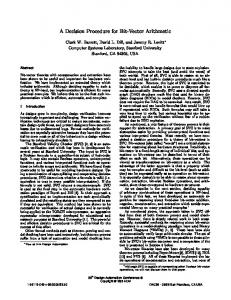
V. Ganesh and D.L. Dill Input Formula

Substitution Simplifications Linear Solving

BitBlast Refinement Array Axioms CNF Conversion

SAT Solver

SAT

UNSAT

Fig. 1. STP Architecture

In more detail, STP’s architecture is depicted in Figure 1. Processing consists of three phases of word-level transformations; followed by conversion to a purely Boolean formula and Boolean simplifications (this process is called “Bit Blasting”); and finally conversion to propositional CNF and solving by a SAT solver. The primary focus of this paper is on word level optimizations for arithmetic, arrays and refinement for arrays. Expressions are represented as directed acyclic graphs (DAGs), from the time they are created by the parser or through the C-interface, until they are converted to CNF. In the DAG representation, isomorphic subtrees are represented by a single node, which may be pointed to by many parent nodes. This representation has advantages and disadvantages, but the overwhelming advantage is compactness. It is possible to identify some design principles that have worked well during the development of STP. The overarching principle is to procrastinate when faced with hard problems. That principle is applied in many ways. Transformations that are risky because they can significantly expand the size of the expression DAG are postponed until other, less risky, transformations are performed, in the hope that the less risky transformation will reduce the size and number of expressions requiring more risky transformations. This approach is particularly helpful for array expressions. Counter-example-guided abstraction/refinement is now a standard paradigm in formal tools, which can be applied in a variety of ways. It is another application of the procrastination principle. For example, the UCLID tool abstracts and refines the precision of integer variables. A major novelty of STP’s implementation is the particular implementation of the refinement loop in Figure 1. In STP, abstraction is implemented (i.e. an abstract formula is obtained) by omitting conjunctive constraints from a concrete formula, where the concrete formula must be equisatisfiable with the original formula. (Logical formulas φ and ψ are equisatisfiable iff φ is satisfiable exactly when ψ is satisfiable.) When testing an abstract formula for satisfiability, there can be three results. First, STP can determine that the abstracted formula is unsatisfiable. In this case, it is clear that the original formula is unsatisfiable, and hence STP can return “unsatisfiable” without additional refinement, potentially saving a massive amount of work. A second possible outcome is that STP finds a satisfying assignment to the abstract formula. In this case, STP converts the satisfying assignment to a (purported) concrete

A Decision Procedure for Bit-Vectors and Arrays

523

model, 1 and also assigns zero to any variables that appear in the original formula but not the abstract formula, and evaluates the original formula with respect to the purported model. If the result of the evaluations is TRUE , the purported model is truly a model of the original formula (i.e. the original formula is indeed satisfiable) and STP returns the model without further refinement iterations. The third possible outcome is that STP finds a purported model, but evaluating the original formula with respect to that model returns FALSE . In that case, STP refines the abstracted formula by heuristically choosing additional conjuncts, at least one of which must be false in the purported model and conjoining those formulas with the abstracted formula to create a new, less abstract formula. In practice, the abstract formula is not modified; instead, the new formulas are bit-blasted, converted to CNF, and added as clauses to the CNF formula derived from the previous abstract formula, and the resulting CNF formula solved by the SAT solver. This process is iterated until a correct result is found, which must occur because, in the worst case, the abstract formula will be made fully concrete by conjoining every formula that was omitted by abstraction. When all formulas are included, the result is guaranteed to be correct because of the equisatisfiability requirement above.

3 Arrays As was mentioned above, arrays are used heavily in software analysis applications, and reasoning about arrays has been a major bottleneck in many examples. STP’s input language supports one-dimensional (non-extensional) arrays [17] that are indexed by bit-vectors and contain bit-vectors. The operations on arrays are read (A, i), which returns the value at location A[i] where A is an array and i is an index expression of the correct type, and write(A, i, v), which returns a new array with the same value as A at all indices except possibly i, where it has the value v. The value of a read is a bitvector, which can appear as an operand to any operation or predicate that operates on bit-vectors. The value of an array variable or an array write has an array type, and may only appear as the first operand of a read or write, or as the then or else operand of an if-then-else. In particular, values of an array type cannot appear in an equality or any other predicate. In the unoptimized mode, STP reduces all formulas to an equisatisfiable form that contains no array read s or writes, using three transformations. (In the following, the expression ite(c1 , e1 , e2 ) is shorthand for if c1 then e1 else e2 endif.) These transformations are all standard. The Ite-lifting transformation converts read (ite(c, write(A, i, v), e), j) to ite(c, read (write(A, i, v), j), e). (There is a similar transformation when the write is in the “else” part of the ite.) The read-over-write transformation eliminates all write terms by transforming read (write(A, i, v), j) to ite(i = j, v, read (A, j)). Finally, the read elimination transformation eliminates read terms by introducing a fresh bit-vector variable for each such expression, and adding more predicates to ensure consistency. Specifically, whenever a term read (A, i) appears, it is replaced by a fresh variable v, and new 1

A model is an assignment of constant values to all of the variables in a formula such that the formula is satisfied.

524

V. Ganesh and D.L. Dill

predicates are conjoined to the formula i = j ⇒ v = w for all variables w introduced in place of read terms read (A, j), having the same array term as first operand. As an example of this transformation, the simple formula (read (A, 0) = 0) ∧ (read (A, i) = 1) would be transformed to v1 = 0 ∧ v2 = 1 ∧ (i = 0 ⇒ v1 = v2 ). The formula of the form (i = 0 ⇒ v1 = v2 ) is called an array read axiom. 3.1 Optimizing Array Reads Read elimination, as described above, expands each formula by up to n(n−1)/2 nodes, where n is the number of syntactically distinct index expressions. Unfortunately, software analysis applications can produce thousands of reads with variable indices, resulting in a lethal blow-up when this transformation is applied. While this blow-up seems unavoidable in the worst case, appropriate procrastination leads to practical solutions for many very large problems. Two optimizations which have been very effective are array substitution and abstraction-refinement for reads, which we call read refinement. The array substitution optimization reduces the number of array variables by substituting out all constraints of the form read (A, c) = e1 , where c is a constant and e1 does not contain another array read. Programs often index into arrays or memory using constant indexes, so this is a case that occurs often in practice. The optimization has two passes. The first pass builds a substitution table with the left-hand-side of each such equation (read (A, c)) as the key and the right-hand-side (e1 ) as the value, and then deletes the equation from the input query. The second pass over the expression replaces each occurrence of a key by the corresponding table entry. Note that for soundness, if a second equation is encountered whose left-hand-side is already in the table, the second equation is not deleted and the table is not changed. For example, if STP saw read (A, c) = e1 then read (A, C) = e2 , the second formula would not be deleted and would later be simplified to e1 = e2 . The second optimization, read refinement, delays the translation of array reads with non-constant indexes in the hope of avoiding read elimination blowup. Its main trick is to solve a less-expensive approximation of the formula, check the result in the original formula, and try again with a more accurate approximation if the result is incorrect. Read formulas are abstracted by performing read elimination, i.e., replacing reads with new variables, but not adding the array read axioms. This abstracted formula is processed by the remaining stages of STP. As discussed in the overview, if the result is unsatisfiable, that result is correct and can be returned immediately from STP. If not, the abstract model found by STP is converted to a concrete model and the original formula is evaluated with respect to that model. If the result is TRUE , the answer is correct and STP returns that model. Otherwise, some of the array read axioms from read elimination are added to the formula and STP is asked to satisfy the modified formula. This iteration repeats until a correct result is found, which is guaranteed to happen (if memory and time are not exhausted) because all of the finitely many array read axioms will eventually be added in the worst case. The choice of which array read axioms to add during refinement is a heuristic that is important to the success of the method. A policy that seems to work well is to find a nonconstant array index term for which at least one axiom is violated, then add all of the violated axioms involving that term. Adding at least one false axiom during refinement

A Decision Procedure for Bit-Vectors and Arrays

525

guarantees that STP will not find the same false model more than once. Adding all the axioms for a particular term seems empirically to be a good compromise between adding just one formula, which results in too many iterations, and adding all formulas, which eliminates all abstraction after the first failure. For example, suppose STP is given the formula (read (A, 0) = 0)∧(read (A, i) = 1). STP would first apply the substitution optimization by deleting read (A, 0) = 0 from the formula, and inserting the pair (read (A, 0), 0) in the substitution table. Then, it would replace read (A, i) by a new variable vi , thus generating the under-constrained formula vi = 1. Suppose STP finds the solution i = 1 and vi = 1. STP then translates the solution to the variables of the original formula to get (read (A, 0) = 0) ∧ read (A, 1) = 1). This solution is satisfiable in the original formula as well, so STP terminates since it has found a true satisfying assignment. However, suppose that STP finds the solution i = 0 and vi = 1. Under this solution, the original formula eventually evaluates to read (A, 0) = 0 ∧ read (A, 0) = 1, which after substitution gives 0 = 1. Hence, the solution to the under-constrained formula is not a solution to the original formula. In this case, STP adds the array read axiom i = 0 ⇒ read (A, i) = read (A, 0). When this formula is checked, the result must be correct because the new formula includes the complete set of array read axioms. 3.2 Optimizing Array Writes Efficiently dealing with array writes is crucial to STP’s utility in software applications, some of which produce deeply nested write terms when there are many successive assignments to indices of the same array. The read-over-write transformation creates a performance bottleneck by destroying sharing of subterms, creating an unacceptable blow-up in DAG size. Consider the simple formula: read (write(A, i, v), j) = read (write(A, i, v), k), in which the write term is shared. The read-over-write transformation translates this to ite(i = j, v, read (A, j)) = ite(i = k, v, read (A, k)). When applied recursively to the deeply nested write terms, it essentially creates a new copy of the entire DAG of write terms for every distinct read index, which exhausts memory in large examples. Once again, the procrastination principle applies. The read-over-write transformation is delayed until after other simplification and solving transformations are performed, except in special cases like read (write(A, i, v), i + 1), where the read and write indices simplify to terms that are always equal or not equal. In practice, the simple transformations convert many index terms to constants. The read-over-write transformation is applied in a subsequent phase. When that happens, the formula is smaller and contains more constants. This simple optimization is enormously effective, enabling STP to solve many very large problems with nested writes that it is otherwise unable to do. Abstraction and refinement can also be used on write expressions, when the previous optimization leaves large numbers of read s and writes, leading to major speed-ups on some large formulas. For this optimization, array read-over-write terms are replaced by new variables to yield a conjunction of formulas that is equisatisfiable to the original set. The example above is transformed to:

526

V. Ganesh and D.L. Dill

v1 = v2 v1 = ite(i = j, v, read (A, j)) v2 = ite(i = k, v, read (A, k)) where the last two formulas are called array write axioms. For the abstraction, the array write axioms are omitted, and the abstracted formula v1 = v2 is processed by the remaining phases of STP. As with array reads, the refinement loop iterates only if STP finds a model of the abstracted formula that is also not a model of the original formula. Write axioms are added to the abstracted formula, and the refinement loop iterates with the additional axioms until a definite result is produced. Although, this technique leads to improvement in certain cases, the primary problem with it is that the number of iterations of the refinement loop is sometimes very large.

4 Linear Solver and Variable Elimination One of the essential features of STP for software analysis applications is its efficient handling of linear twos-complement arithmetic. The heart of this is an on-the-fly solver. The main goal of the solver is to eliminate as many bits of as many variables as possible, to reduce the size of the transformed problem for the SAT solver. In addition, it enables many other simplifications, and can solve purely linear problems outright, so that the SAT solver does not need to be used. The solver solves for one equation for one variable at a time. That variable can then be eliminated by substitution in the rest of the formula, whether the variable occurs in linear equations or other formulas. In some cases, it cannot solve an entire variable, so it solves for some of the low-order bits of the variable. After bit-blasting, these bits will not appear as variables in the problem presented to the SAT solver. Non-linear or wordlevel terms (extracts, concats etc.) appearing in linear equations are treated as bit-vector variables. The algorithm has worst-case time running time of O(k 2 n) multiplications, where k is the number of equations and n is the number of variables in the input system of linear bit-vector equations.2 If the input is unsatisfiable the solver terminates with FALSE . If the input is satisfiable it terminates with a set of equations in solved form, which symbolically represent all possible satisfying assignments to the input equations. So, in the special case where the formula is a system of linear equations, the solver leads to a sound and complete polynomial-time decision procedure. Furthermore, the equations are reduced to a closed form that captures all of the possible solutions. Definition 1. Solved Form: A list of equations is in solved form if the following invariants hold over the equations in the list. 2

As observed in [4], the theory of linear mod 2n arithmetic (equations only) in tandem with concatenate and extract operations is NP-complete. Although STP has concatenate and extraction operations, terms with those operations are treated as independent variables in the linear solving process, which is polynomial. A hard NP-complete input problem constructed out of linear operations, concatenate and extract operations will not be solved completely by linear solving, and will result in work for the SAT solver.

A Decision Procedure for Bit-Vectors and Arrays

527

1) Each equation in the list is of the form x[i : 0] = t or x = t, where x is a variable and t is a linear combination of the variables or constant times a variable (or extractions thereof) occuring in the equations of the list, except x 2) Variables on the left hand side of the equations occuring earlier in the list may not occur on the right hand side of subsequent equations. Also, there may not be two equations with the same left hand side in the list 3) If extractions of variables occur in the list, then they must always be of the form x[i : 0], i.e. the lower extraction index must be 0, and all extractions must be of the same length 4) If an extraction of a variable x[i : 0] = t occurs in the list, then an entry is made in the list for x = x1 @t, where x1 is a new variable refering to the top bits of x and @ is the concatenation symbol The algorithm is illustrated on the following system: 3x + 4y + 2z = 0 2x + 2y + 2 = 0 4y + 2x + 2z = 0 where all constants, variables and functions are 3 bits long. The solver proceeds by first choosing an equation and always checks if the chosen equation is solvable. It uses the following theorem from basic number theory to detern ai xi = ci mod 2b is solvable for the unknowns xi mine if an equation is solvable: Σi=1 if and only if the greatest common divisor of {a1 , . . . , an , 2b } divides ci . In the example above, the solver chooses 3x + 4y + 2z = 0 which is solvable since the gcd(3, 4, 2, 23) does indeed divide 0. It is also a basic result from number theory that a number a has a multiplicative inverse mod m iff gcd(a, m) = 1, and that this inverse can be computed by the extended greatest-common divisor algorithm [8] or a method from [4]. So, if there is a variable with an odd coefficient, the solver isolates it on the left-hand-side and multiplies through by the inverse of the coefficient. In the example, the multiplicative inverse of 3 mod 8 is also 3, so 3x + 4y + 2z = 0 can be solved to yield x = 4y + 6z. Substituting 4y + 6z for x in the remaining two equations yields the system 2y + 4z + 2 = 0 4y + 6z = 0 where all coefficients are even. Note that even coefficients do not have multiplicative inverses in arithmetic mod 2b , and, hence we cannot isolate a variable. However, it is possible to solve for some bits of the remaining variables. The solver transforms the whole system of solvable equations into a system which has at least one summand with an odd coefficient. To do this, the solver chooses an equation which has a summand whose coefficient has the minimum number of factors of 2. In the example, this would the equation 2y + 4z + 2 = 0, and the summand would be 2y. The whole system is divided by 2, and the high-order bit of each variable is dropped, to obtain a reduced set of equations

528

V. Ganesh and D.L. Dill

y[1 : 0] + 2z[1 : 0] + 1 = 0 2y[1 : 0] + 3z[1 : 0] = 0 where all constants, variables and operations are 2 bits. Next, y[1 : 0] is solved for to obtain y[1 : 0] = 2z[1 : 0] + 3. Substituting for y[1 : 0] in the system yields a new system of equations 3z[1 : 0] + 2 = 0. This equation can be solved for z[1 : 0] to obtain z[1 : 0] = 2. It follows that original system of equations is satisfiable. It is important to note here that the bits y[2 : 1] and z[2 : 1] are unconstrained. The solved form in this case is x = 4y + 6z ∧ y[1 : 0] = 2z[1 : 0] + 3 ∧ z[1 : 0] = 2 (Note that in the last two equations all variables, constants and functions are 2 bits long). Algorithms for deciding the satisfiability of a system of equations and congruences in modular or residue arithmetic have been well-known for a long time. However, most of these algorithms do not provide a solved form that captures all possible solutions. Some of the ideas presented here were devised by Clark Barrett and implemented in the SVC decision procedure [12,4], but the SVC algorithm has exponential worst-case time complexity while STP’s linear solver is polynomial in the worst-case. The closest related work is probably in a paper by Huang and Cheng [12], which reduces a set of equations to a solved form by Guassian elimination. On the other hand, STP implements an online solving and substitution algorithm that gives a closed form solution. Such algorithms are easier to integrate into complex decision procedures.

5 Experimental Results This section presents empirical results on large examples from software analysis tools, and on randomly generated sets of linear equations. The effects of abstraction and linear solving in STP are examined. It is difficult to compare STP with other decision procedures, because no publicly available decision procedures except CVCL (from the authors research group) can deal with terms involving both bit-vectors and arrays indexed by bit-vectors. CVCL is hopelessly inefficient compared with STP, which was written to replace it. Terms in Yices can include bit-vectors and uninterpreted functions over bit-vectors. Uninterpreted functions are equivalent to arrays with no write operations, so it is possible to compare the performance of STP and Yices on examples with linear arithmetic and one realistic example with a read-only array. In Table 1, STP is compared with all optimizations on (All ON), Array Optimizations on (Arr-ON,Lin-OFF), linear-solving on (Arr-OFF,Lin-ON), and all optimizations off (ALL OFF) on the BigArray examples (these examples are heavy on linear arithmetic and array reads). Table 2 summarizes STP’s performance, with and without array write abstraction, on the big array examples with deeply nested writes. Table 3 compares STP with Yices on a very small version of a BigArray example, and some randomly generated linear system of equations. All experiments were run on a 3.2GHz/2GB RAM Intel machine running Linux. Table 1 includes some of the hardest of the BigArray examples which are usually tens of megabytes of text, typically hundreds of thousands of 32 bit bit-vector variables, lots of array reads, and large number of linear constraints derived from [14,16]. The primary reason for timeouts is an out-of-memory exception. Table 1 shows that all optimizations

A Decision Procedure for Bit-Vectors and Arrays

529

Table 1. STP performance in different modes over BigArray Examples. Names are followed by the nodesize. Approximate node size is in millions of nodes. 1M is one million nodes. Shared nodes are counted exactly once. NR stands for No Result. All timings are in seconds. MO stands for out of memory error. These examples were generated using the CATCHCONV tool. Example Name (Node Size) testcase15 (0.9M) testcase16 (0.9M) thumbnailout-spin1 (3.2M) thumbnailout-spin1-2 (4.3M) thumbnailout-noarg (2.7M)

Result sat sat sat NR sat

All ON 66 67 115 MO 840

Arr-ON,Lin-OFF Arr-OFF,Lin-ON All OFF 192 64 MO 233 66 MO 111 113 MO MO MO MO MO 840 MO

Table 2. STP performance in different modes over BigArray Examples with deep nested writes. Names are followed by the nodesize. 1M is one million nodes (1K is thousand nodes). Shared nodes are counted exactly once. NR stands for No Result. All timings are in seconds. MO stands for out of memory error.These examples were generated using the CATCHCONV and Minesweeper tools. Example Name (Node Size) grep0084 (69K) grep0095 (69K) grep0106 (69K) grep0117 (70K) grep0777 (73K) 610dd9dc (15K) testcase20 (1.2M)

Result sat sat sat sat NR sat sat

WRITE Abstraction 109 115 270 218 MO 188 67

NO WRITE Abstraction 506 84 > 600 > 600 MO 101 MO

are required for solving the hardest real-world problems. As expected, STP’s linear solver is very helpful in solving these examples. Table 2 includes examples with deeply nested array writes and modest amounts of linear constraints derived from various applications. The “grep” examples were generated using the Minesweeper tool while trying to find bugs in unix grep program. The 610dd9c formula is generated by a Minesweeper analysis of a program that is used in “botnet” attack. The formula testcase20 was generated by CATCHCONV. As expected, STP with write abstraction-refinement ON can yield a very large improvement over STP with write abstraction-refinement switched OFF, although it is not always faster. Yices and STP were also compared on small, randomly-generated systems of linear equations with coefficients ranging from 1 to 216 , from 4 to 256 variables of 32 bits each, and 4 to 256 equations. Yices consistently timed out at 200 seconds on examples with 32 or more variables, and was significantly slower than STP on the smaller examples. The hardest problem for STP in this set of benchmarks was a test case with 32 equations and 256 variables of 32 bits, which STP solved in 90 seconds. There are two cases for illustration in Table 3. Yices times out on even a 50 variable 50 equation example, and when it does finish it is much slower than STP. There is one large, real example with read-only arrays, linear arithmetic and bitvectors which is suitable for comparison with Yices. On this example, Yices is nearly

530

V. Ganesh and D.L. Dill

Table 3. STP vs. Yices. Timeout per example: 600sec. The last example was generated using the Replayer tool. Example 25 var/25 equations(unsat) 50 var/50 equations(sat) cookie checksum example(sat)

STP Yices 0.8s 42s 13s TimeOut 2.6s 218s

one hundred times slower than STP. Unfortunately, we could not compare Yices with STP on examples with array writes since Yices does not support array writes with bit-vector indexing. More meaningful comparisons will have to wait till competing decision procedures includes bit-vector operations and a theory of arrays indexed by bitvectors. All tests in this section are available at http://verify.stanford.edu/ stp.html

6 Conclusion Software applications such as program analysis, bug finding, and symbolic simulation of software tend to impose different conditions on decision procedures than hardware applications. In particular, arrays become a bottleneck. Also, the constraints tend to be very large with lots of linear bit-vector arithmetic in them. Abstraction-refinement algorithms is often helpful for handling large array terms. Also, the approach of doing phased word-level transformations, starting with the least expensive and risky transformations, followed by translation to SAT seems like a good design for decision procedures for the applications considered. Finally, linear solving, when implemented carefully, is effective in variable elimination.

Acknowledgements We are indebted to the following users for their feedback and for great examples: David Molnar from Berkeley; Cristian Cadar, Dawson Engler and Aaron Bradley from Stanford; Jim Newsome, David Brumley, Ivan Jaeger and Dawn Song from CMU; This research was supported by Department of Homeland Security (DHS) grant FA8750-05-2-0142 and by National Science Foundation grant CNS-0524155. Any opinions, findings, and conclusions or recommendations expressed in this material are those of the author and do not necessarily reflect the view of the Department of Homeland Security or the National Science Foundation.

References 1. SMTLIB website: http://www.csl.sri.com/users/demoura/smt-comp/ 2. Barrett, C., Berezin, S.: CVC Lite: A new implementation of the cooperating validity checker. In: Alur, R., Peled, D.A. (eds.) CAV 2004. LNCS, vol. 3114, Springer, Heidelberg (2004)

A Decision Procedure for Bit-Vectors and Arrays

531

3. Barrett, C., Dill, D., Levitt, J.: Validity checking for combinations of theories with equality (Palo Alto, California, November 6–8). In: Srivas, M., Camilleri, A. (eds.) FMCAD 1996. LNCS, vol. 1166, pp. 187–201. Springer, Heidelberg (1996) 4. Barrett, C.W., Dill, D.L., Levitt, J.R.: A decision procedure for bit-vector arithmetic. In: Proceedings of the 35th Design Automation Conference, San Francisco, CA (June 1998) 5. Brumley, D., Hartwig, C., Liang, Z., Newsome, J., Song, D., Yin, H.: Towards automatically identifying trigger-based behavior in malware using symbolic execution and binary analysis. Technical Report CMU-CS-07-105, Carnegie Mellon University School of Computer Science (January 2007) 6. Bryant, R.E., Kroening, D., Ouaknine, J., Seshia, S.A., Strichman, O., Brady, B.: Deciding bit-vector arithmetic with abstraction. In: 13th Intl. Conference on Tools and Algorithms for the Construction of Systems (TACAS) (2007) 7. Cadar, C., Ganesh, V., Pawlowski, P., Dill, D., Engler, D.: EXE: Automatically generating inputs of death. In: Proceedings of the 13th ACM Conference on Computer and Communications Security, ACM Press, New York (October-November 2006) 8. Cormen, T.H., Leiserson, C.E., Rivest, R.L.: Introduction to Algorithms (chapter 11), pp. 820–825. MIT Press, Cambridge (1998) 9. Dutertre, B., de Moura, L.: A Fast Linear-Arithmetic Solver for DPLL(T). In: Ball, T., Jones, R.B. (eds.) CAV 2006. LNCS, vol. 4144, pp. 81–94. Springer, Heidelberg (2006) 10. Een, N., Sorensson, N.: An extensible sat-solver. In: Proc. Sixth International Conference on Theory and Applications of Satisfiability Testing, May 2003, pp. 78–92 (May 2003) 11. Ganzinger, H., Hagen, G., Nieuwenhuis, R., Oliveras, A., Tinelli, C.: Dpll(t): Fast decision procedures (2004) 12. Huang, C., Cheng, K.: Assertion checking by combined word-level atpg and modular arithmetic constraint-solving techniques. In: Design Automation Conference (DAC), pp. 118–123 (2001) 13. Lahiri, S.K., Seshia, S.A.: The uclid decision procedure. In: Alur, R., Peled, D.A. (eds.) CAV 2004. LNCS, vol. 3114, pp. 475–478. Springer, Heidelberg (2004) 14. Molnar, D., Wagner, D., Seshia, S.A.: Catchconv: A tool for catching conversion errors. Personal Communications (2007) 15. Nelson, G., Oppen, D.C.: Simplification by cooperating decision procedures. ACM Transactions on Programming Languages and Systems 1(2), 245–257 (1979) 16. Newsome, J., Brumley, D., Franklin, J., Song, D.: Replayer: Automatic protocol replay by binary analysis. In: The Proceedings of the 13th ACM Conference on Computer and and Communications Security (CCS), ACM Press, New York (2006) 17. Stump, A., Barrett, C., Dill, D., Levitt, J.: A Decision Procedure for an Extensional Theory of Arrays. In: 16th IEEE Symposium on Logic in Computer Science, pp. 29–37. IEEE Computer Society Press, Los Alamitos (2001) 18. Stump, A., Barrett, C.W., Dill, D.L.: Cvc: A cooperating validity checker. In: Brinksma, E., Larsen, K.G. (eds.) CAV 2002. LNCS, vol. 2404, pp. 500–504. Springer, Heidelberg (2002)