a decision support system for complex ... - Semantic Scholar

IEEE:TRANSACTIONS ON SYSTEMS, MAN, A N D C’YBLRNFTICS,VOL.

20, NO. 4, J U L . Y / A ~ J G ~ J S1990 T

745

MGA: A Decision Support System for Complex, Incompletely Defined Problems E. DOWNEY BRILL, JR., JOHN M. FLACH, ASSOCIATE MEMBER, LEWIS D. HOPKINS, AND S . RANJITHAN

Abstract -Modeling-to-generate alternatives (MGA) is a technique for using mathematical programming models to generate a small number of different solutions for the decision maker to consider when dealing with complex, incompletely defined problems. The logic of MGA is presented in the context of concerns about the limitations of mathematical models and limitations of the human decisionmakers who use them. Arguments and experimental evidence are presented to support the assumption that the human-machine decisionmaking system will perform better when the human is presented with a few, different alternatives than when presented a homogeneous set of alternatives as might result from sensitivity analysis.

IEEE,

ing and solving complex problems is very small compared with the size of the problems.” The common theme that is emerging from the concerns of these two communities is that the challenge in designing decision support systems is “how to ‘couple’ human intelligence and machine power in a single integrated system that maximizes joint performance” [38]. This paper will present one approach that shows promise as an effective technique for coupling humans and mathematical models. Modeling-to-generate alternatives (MGA) is a technique in which mathematical programming models are INTRODUCTION applied to complex, incompletely defined problems to COMMON THEME is emerging from two commuproduce a small number of different alternatives. These nities concerned about the effectiveness of decision alternatives provide initial conditions for the human decisystems for solving complex problems. The operations sionmaker who must ultimately choose a solution that research/management science community [2] has focused best satisfies the “real world” problem. MGA is an examon the limitations of mathematical models for providing ple of a “joint cognitive systems” [38] approach to deci“the answer” to complex problems. Concern for these sion support systems. The joint cognitive systems aplimitations has led to the conclusion that the role of proach focuses on the combination of the human and mathematical models should not be to provide “the machine (i.e., optimization algorithms or models generally answer”; the role should be to provide “intuition, inimplemented on computers) as a decisionmaking system. sight, and understanding that supplements that of the This holistic approach recognizes that the human and the decisionmakers” [2], [20]. A second community, the engimachine both bring abilities and limitations to the comneering/cognitive psychology community has focused on plex problem. The abilities of one element can complethe limitations that the human brings to decision systems ment those of the other, compensating for limitations, [14]. For example, Reason [26] quotes Simon [31] who leading to greater performance than can be expected notes that “the capacity of the human mind for formulatfrom either element alone; or the limitations can be compounded with performance at best as good as the Manuscript received March 3, 1989; revised August 12, 1989 and strongest element, and possibly much worse than either March 6, 1990. This work was supported in part by a grant from the element alone (1331). Decision, Risk, and Management Science Program of the National The MGA approach is based on several important Science Foundation, Grant Number NSF FES 85-10274. S . Ranjithan was supported by the U S . Army Construction Research Laboratory for assumptions about the joint cognitive system. First, it is the last year of this project, and in part by the Department of Civil assumed that the solutions to mathematical programming Engineering, University of Illinois, Urbana-Champaign. E . D. Brill, Jr. is at the Department of Civil Engineering. North models will seldom represent the best solutions to actual Carolina State University, Raleigh, NC, 61200. complex problems. For a host of reasons, some attributes J. M. Flach was with the Department of Mechanical and Industrial of the actual problem will not be represented in the Engineering, University of Illinois at Urbana-Champaign, 144 Mechanical Engineering Building. 1206 West Green Street, Urbana, IL 61801. mathematical model. Solutions to mathematical models He is now with the Armstrong Aerospace Medical Research Laboratory, provide input for the human decisionmaker who must Wright-Patterson Air Force Base, OH. integrate information from additional sources before L. D. Hopkins is with the Department of Urban and Regional Planning, University of Illinois at Urbana-Champaign, 1003 W. Nevada, choosing the solution for the real problem. Urbana, IL, 61801 A second assumption of the MGA approach is that the S . Ranjithan is with the Department of Civil Engineering, University human’s ability to appropriately integrate the data reof Illinois at Urbana-Champaign, Urbana, IL. 61801. ceived from the model with other sources of information IEEE Log Number 9035714.

A

0018-9472/90/07OO-0745$01 .0O 01990 IEEE

746

IEEE TRANSACTIONS ON SYSTEMS, MAN, AND CYBERNETICS, VOL.

will be affected by two attributes of the model output. The first attribute is the number of alternatives provided. It is assumed that a small (3 to 10) number of alternatives will be best. The second attribute is the degree of difference among alternatives. The MGA approach is based on the hypothesis that performance will be best when the degree of difference among alternatives is greatest. This paper begins with a discussion of the contributions and limitations of two key elements within the decision system-the mathematical programming model and the human. It continues with a discussion of how MGA is designed to blend these elements into an effective system. Finally, an empirical test of the assumptions underlying the MGA approach is presented.

20, NO. 4, JULY/AUGUST 1990

lnfenor Region

i Optimal

(b) . ,

Mathematical Programming Models

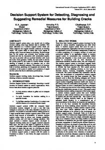
Mathematical programming models identify an “optimal” solution with respect to an objective, subject to constraints. Multiple objective methods, in addition, generally provide tools to assist decisionmakers to explore the set of noninferior solutions so that value judgments about trade-offs among modeled objectives can be evaluated. A fundamental limitation in using mathematical programming models in complex decision environments is that they are seldom a complete representation of the problem 121, ill], 1201, [241, [271, [291, [351. Modeling methods limit the number of dimensions that can be included. Important issues may be left out of mathematical models because of difficulty in quantifying them. Also, limitations in the modeler’s understanding of the problem may result in important dimensions being left out. The result is that the solutions of mathematical programming models will be “optimal” or “noninferior” only with respect to a “small world” [281 representation of the problem. The consequences of this small world representation are illustrated in Fig. 1, which is adapted from Brill [2]. Fig. l(a) illustrates the objective space for a one-dimensional (1-D) model of the problem. A mathematical programming model can be used to find the “optimal” solution given the objective space and a set of constraints. Fig. l(b) illustrates a mathematical programming solution to the same problem, but with a second objective included in the model. Note that if there are compromises in meeting the two objectives, no matter what the shape of the noninferior surface, the new “optimal” solution will always project to the inferior set from the l-D model. If it were assumed that the first dimension is more important than the second, then the new optimal solution will likely be in the general area of the optimal solution to the one-dimensional model. Fig. l(c) extends the illustration to a third dimension. Once again, the optimal solution to the expanded model would be found in the inferior region of the two-dimensional model. Again, if it were assumed that the third dimension (2-D) is less important than the previous two, the optimal solution would likely be in the vicinity of the solution to the 2-D model. Thus, whenever the objective

(C) Fig. 1 . Illustration showing that optimal solution to a simple model will project to inferior region in objective space when additional dimensions are included in model. (a) 1-D solution space. (b) 2-D solution space. (c) 3-D solution space.

space for a mathematical programming model has fewer dimensions than the problem being considered, the solution to the problem will generally be found in the inferior region of the modeled solutions. However, if the most important dimension or dimensions are included in the model, then the problem solution is likely to be in the region of the optimal solution to the model. The region near the optimal solution or noninferior surface provides a promising area for exploration of the actual problem space. The success of the joint cognitive system will depend on the human’s ability to search the “inferior set” of model solutions to find the best solution whenever the complexity of the actual problem exceeds the complexity of the model. Human Decisionmaking In working on ill-defined problems the human operator must make observations (i.e. collect data), generate hypotheses based on this data, and finally make a decision. This is a highly iterative process with observations providing the basis for hypotheses and hypotheses guiding and constraining observations. As with any iterative process a key to success will be the stopping rule. How many hypotheses should be considered? How much data is enough? A less than satisfactory decision may be made because the appropriate hypothesis was not generated or because insufficient data were sampled. On the other hand, resources may be squandered in generating hypotheses that have extremely low probabilities of being appropriate or in collecting far more data than is required to make a good decision. Hypothesis Generation: Corbin [7, p. 521 describes how information is extracted from alternatives in experiments

BRILL

et al.: MGA-A

DECISION SUPPORT SYSTEM

with the ill-defined “secretary problem,” in which a number of choice alternatives is sequentially presented and the decisionmaker may stop and select one of the currently available offers, or take another observation at some cost. She reports that “subjects seek to extract information from the alternatives as they are sequentially observed, and to formulate hypotheses about the underlying distributions that govern them.” The criteria (hypotheses about what makes a good secretary) are not fixed, but dynamically evolve in the course of manipulating the problem. Corbin [7, p. 521 illustrates the role of alternatives in shaping hypotheses with the following anecdote. “Consider a manager interviewing potential secretaries, uncertain of what criterion to use in deciding among them. One candidate smokes so much during the interview that it occurs to the manager how unpleasant smoke might make the office. Thus, how much a candidate smokes becomes a criterion for the eventual decision that is incorporated into the chooser’s goals.” Gettys and Fisher [12] have proposed a model for the process of generating hypotheses for ill-defined problems. In their model generating hypotheses is an intermittent process. The decision to generate new hypotheses is based on the plausibility of the current hypotheses set. If observed data is consistent with hypotheses in the current set, no new hypotheses will be generated. Gettys and Fisher note that this strategy is similar to the “win-stay, lose-shift” strategy that has been described in the context of concept identification tasks. New hypotheses are generated only when “current hypotheses are made less plausible by data” [12, p. 1041. Gettys and Fisher conclude that “this strategy, while nonoptimal, is a heuristic that reduces the information-processing load on the subject.” In addition to the decision to generate hypotheses, a second decision modeled by Gettys and Fisher [12] is the decision about whether or not to add a candidate hypothesis to the set of hypotheses being considered. Two factors which influence this decision are the relative plausibility of the newly generated hypothesis and the size of the current hypothesis set. Gettys and Fisher report that subjects only entertain “hypotheses that are strong competitors with their best hypothesis, and they usually require a new hypothesis to be at least half as likely as their best hypothesis before incorporating it into their current hypothesis set.” They also noted a tendency for the relative plausibility threshhold to become more strict as the size of the current hypothesis set becomes large. Observation of Datu: In Gettys and Fisher’s [121 research the subject was responsible for generating hypotheses, but the experimenter controlled observations of data. However, in operational decision systems the human is responsible for generating and evaluating hypotheses as well as for selecting the data to be observed. Much research has focused on the processes involved in selecting and observing data to evaluate a fixed set of hypotheses. This research has revealed a tendency toward “cognitive hysteresis.” Norman [22] describes cognitive

747

hysteresis as a tendency to “stick with a decision beyond the point where the situation would otherwise warrant it” (p. 132). An important dimension of this cognitive hysteresis has been a tendency, identified by Wason 1361, E371, for humans to bias their search toward confirming evidence. Norman [22, p. 321 notes that “this bias holds despite the fact that confirmation is often a weak source of evidence whereas a search for negative evidence would provide quite efficient tests of the hypothesis.” Klayman and Ha [17, p. 2111 have written an extensive review examining the issues of confirmation, disconfirmation, and information in hypothesis testing by human decjsionmakers. They argue that rather than a bias toward4 seeking confirmation of hypotheses, people tend to adopt a “positive test strategy.” That is, people tend to “test cases that are expected (or known) to have the property of interest, rather than those expected (or known) to lack that property.” They argue that unlike a confirmation bias with its negative connotation of irrationality, a positive test strategy “can be a very good heuristic for determining the truth or falsity of a hypothesis under realistic conditions.” This is particularly true when the base rate of positive events is low. That is, when the number of cases expected to have the property of interest is an order of magnitude less than the number of cases expected to lack the property. Klayman and Ha [17] argue that “real-world hypothesis testing most often concerns minority phenomena.” However, this positive test strategy is a heuristic and therefore can sometimes lead to errors or inefficiencies. In addition to confirmation bias and/or a positive test bias, other examples of cognitive hysteresis can be found in the psychological literature. These examples include “functional fixedness” [8], “conservatism” [91, and the “anchoring and adjustment heuristic” [34]. Each of these examples illustrates the critical constraints that early information can have on human decisionmaking and problem solving. Thus, the human decisionmakers can introduce limitations into decisionmaking systems by constraining the range of hypotheses generated and the range of data that is observed. The following statement from Fischhoff [lo, p. 641 amply characterizes these limitations: “When they think of action options, people often neglect seemingly obvious candidates. Moreover, they seem relatively insensitive to the number or importance of the omitted alternatives.. . . Options that would otherwise command attention are out of mind when they are out of sight, leaving people with the impression that they have analyzed problems more thoroughly than is actually the case.

Hogarth [ 131 has suggested that one solution to this “cognitive myopia” is to pay more attention to the development of imagination and creativity when training decisionmakers. He also cites work by Campbell [4] that suggests that “thought trials” to induce “random variations” may be critical for creative processes such as generating hypotheses.

748

IEEE TRANSACTIONS ON SYSTEMS, MAN, AND CYBERNETICS, VOL.

Recent experimental work by Sniezek and Henry [32, p. 201 on group decisionmaking suggests an additional avenue for minimizing the negative effects due to cognitive hysteresis/myopia. They found that 30% of the time the group judgment was more accurate than the most accurate judgment made by an individual within the group. An important factor for producing this improvement was the amount of disagreement among the individuals. Sniezek and Henry report that “groups with relatively larger variances in their distribution of individual judgments showed more improvement over average individual accuracy,” They further note that “the more disagreement that group members reported, the more accurate were their group judgments.” Thus, thought trials may be one source of random variations critical to stimulating creative processes and expanding the horizons of the human decisionmakers. Another source may be colleagues (e.g., group members of a design team). This paper explores a third approach. That is, the use of operations research models for generating alternatives. THEMGA RESEARCH PROGRAM The MGA research program was motivated by the observation that traditional approaches for using models to support decisionmaking in complex problem domains increased the tendency toward cognitive myopia. That is, the “toy world” solutions provided by mathematical models would tend to inappropriately constrain the range of hypotheses considered by the decisionmakers. The MGA technique is an attempt to exploit the power of mathematical models for screening the many “bad” alternatives from the set of hypotheses to be considered, without inducing a myopic attachment to an oversimplified answer. This is accomplished by generating a few alternatives that are “good” with respect to the modeled objective and that are different with respect to salient dimensions of the solution space. The research program studying the MGA approach is now in its third phase. The first phase of the program focused on the development of algorithms that could be used to generate small sets of alternatives that are feasible, good with respect to modeled objectives, and different from each other. Two general types of algorithms have been found to be most effective for generating alternatives: 1) algorithms based on random generation and 2) algorithms based on maximizing difference as an objective function. Chang, Brill, and Hopkins [5], [6] have developed a random selection process that efficiently obtains solutions that are feasible; that meet specified targets on modeled objectives; and that are different from each other in decision space. Brill [2], [3] suggested an algorithm for maximizing differences called Hop, Skip, and Jump (HSJ). The HSJ method is applicable to linear, mixed integer, or nonlinear programs. It operates by minimizing the sum of the positive valued decision variables from one solution sub-

20, NO. 4, JULY/AUGUST 1990

ject to the original constraints as well as constraints on target values of the known objectives. This procedure tends to drive all current choices out of the subsequent solution and thus forces new choices in. The procedure ‘continues in iterative fashion; at each step the procedure attempts to drive the choices associated with all previous solutions out and force new ones in. Recently, the HSJ approach has been generalized using vector space theory E181, [191. The MGA approach has also been applied to dynamic programming problems [16] through a generalization of Bellman and Kalaba’s [l] Kth shortest path algorithm. By incorporating the difference measure in a weighted objective function, a solution procedure is obtained that is more efficient for MGA purposes than the traditional constraint approach to finding next shortest paths. The second phase of the MGA research program has involved applying these algorithms to complex decision problems to verify that solutions can be generated that are different in interesting ways. The MGA approach (HSJ and random methods) has been applied to land use planning problems formulated as a system of linear relationships [3], [5]. It was found that the algorithms produced several alternatives that were good with respect to the modeled objectives and clearly widely different in spatial configuration. Not only were uses assigned to different zones, but the degree to which use was concentrated in one zone or spread among many zones also varied. The HSJ technique has also been applied to a waste water treatment problem. The technique generated alternatives with significantly different regional configurations [6]. A dynamic programming version has been applied to a flood plain management problem [161. Again, it was found to generate alternatives that were different in interesting ways (e.g. in terms of regions available for urban development and final outflows at the base of the watershed). Thus, techniques for generating small sets of alternatives that are different have been developed. These techniques have been tested and have been shown to be applicable to several realistic, complex problems. However, the motivating assumption behind the development of MGA has yet to be tested in the context of a complex decision problem. The assumption is that the provision of a small number of alternatives that are “different” will lead to better decisions than are typically achieved using traditional approaches to modeling (e.g. optimization and sensitivity analysis). The following section reports a recent experimental test of this assumption.

EXPERIMENT The number of alternatives generated by the MGA approach is small (3-lo), not because of constraints of the techniques, but because of the limited capacity of the human cognitive system. The alternatives are chosen to be “different” to minimize the effects due to “cognitive hysteresis” or “cognitive myopia.” The assumption is that

BRILL

et al.: MGA-A

DECISION SUPPORT SYSTEM

749

Pease select a netwom to m m f y

BOS

80s

Taal Cost X Utilnatlon

Slapovers

Taal Cost % Utilualnn

Slapovers

RECORD FINAL NETWORK

Fig. 2. Initial display for Group 2 containing 4 solutions generated using sensitivity analysis. Each quadrant in left portion of display contains solution. Routes between cities are shown as links. Width of a link is proportional to flow through that link. Cost for each link is also indicated. Circles at each airport represent full capacity. Dark shading represents proportion of trips originating or terminating at airport. Lighter shading indicates additional proportion of passengers passing through airport. Three quantifiable objectives are represented. These are total cost, utilization (congestion) for the two most congested airports, and the proportion of trips having 0, 1, 2, 3 or more stopovers. Subjects are able to modify solutions using commands on upper right of display. Immediate feedback on all dimensions was provided following any change.

the human will consider and test a wider range of hypotheses when given “different” alternatives than when given a single alternative or a homogeneous set of alternatives. A n airline network problem, adapted from earlier work by O’Kelly [231, was chosen as the experimental task for testing MGA. The task was for subjects to develop the best routing for a given matrix of air travel demand among pairs of cities. The problem is presented in diagrammatic form in Fig. 2 that shows a sample screen image as it was presented to subjects. Subjects could change which flight routes would exist in the networks so as to trade off cost, number of stopovers, congestion, and other attributes.

Method Design: Table I shows a factorial combination of three levels of difference (low, medium, and high) with three different numbers of alternatives (1, 4 and 15). Five cells from the matrix resulting from this combination were included in the experiment. Each of the indicated cells represents a different set of initial conditions for decisionmakers. These cells span all levels of the two attributes: size and difference. Difference between two networks is operationally defined as the sum of the absolute differences of passenger-trips per year in each link. The difference measure of a network with respect to a set of (at least two) networks is then computed as the minimum of

TABLE I SUBJECT GROUPS Degree of Difference

Number of Alternatives One

LOW Medium High

G1

Few (4)

Many (15)

G2 (566.5) G3 (1083.4) G4 (2085.1)

**

** G5

all the difference measures between this network and each other network in that set. The level of difference of a set of alternatives was calculated as the sequential sum of the difference measures of each network included in a set. The numbers in parenthesis in Table I are the difference measures in units of thousands of passenger-trips per year for each experimental group. The experiment employed a between subjects design with five experimental groups, corresponding to the cells shown in Table I. Each cell represents a different set of initial conditions for the decisionmakers. The groups were as follows. Group I: This group started with the single alternative that was the least cost solution to the mathematical programming model. The model used was a zero one formulation (see Brill et al. [4]), solved using a branch and bound algorithm on a CRAY X-MP/48 interfaced with a VAX 11/785.

750

IEEE TRANSACTIONS ON SYSTEMS, MAN, AND CYBERNETICS, VOL.

’lease Select a network to modify.

TOPLEFT

00s

I

20, NO. 4, JULY/AUGUST 1990

TOPRIGHT

I BOTTOM LEFT^ BOTTOM RIG^ [

c (

ADDLINE DELETE LINE REROUTE

](-

] e m

)(-

mimost

Lrighl “GKUp2.

Total Cost % Uliluatm

StopoverS

80s

-

Total Cost % Uttluatwn

StopoV0rJ

CANCEL

Fig. 3. Initial display for Group 3 containing four alternatives generated randomly.

Group 2: This group started with four alternative networks. These included the least cost network and three networks derived from it using sensitivity analysis. The value of the difference measure for this group was 566.50 thousand passenger-trips per year. Group 3: This group st irted with four alternatives. These included the least coTit network and three alternatives randomly selected fro n among the set of networks with costs within 10% of the least cost. The value of the difference measure for this group was 1083.39 thousand passenger-trips per year. Group 4: This group also started with four alternatives. These included the least cost network and three alternatives generated using the HSJ technique. The value of the difference measure for this group was 2085.08 thousand passenger trips per year. Group 5: This group started with 15 alternatives. These included the four alternatives from Group 4 plus 11 additional networks generated using the HSJ technique.

The five groups chosen allow a comparison across three levels of difference among alternatives at a fixed number of alternatives (4). This allows a test of the hypothesis that performance will improve when the human operator is provided with alternatives that are maximally different. Thus, it was predicted that Group 4 should perform better than Group 3 and that performance of Group 3 should be superior to that of Group 2. The design also allows a comparison across number of alternatives at the maximum degree of difference for each level. Here the hypothesis was that the addition of different alternatives will result in improved performance only up to some small number, reflecting the limited capacity of the human decisionmakers. Thus, performance of Group 4 should be superior to performance of Group 1 (too few alternatives) and performance of Group 5 (too many alternatives). Given the joint impact of number of alternatives and degree of difference, superior performance was expected for Group 4 (few, different alternatives). Intermediate Figs. 2, 3, and 4 show the initial interface configura- levels of performance were expected for Groups 3 (few, tions for the five experimental groups. Group 1 started less different alternatives) and 5 (too many different alterwith only the minimum cost solution displayed. This net- natives). Finally, the performances of Groups 1 and 2 (low work is shown as the upper left hand network in all three difference among alternatives) were expected to be of figures. Group 2 started with the four solutions shown in lesser quality. Fig. 2. Group 3 started with the four solutions shown in In this experiment both quality of the method and Fig. 3. Fig. 4 shows the starting solutions for Group 4. quality of the solution were evaluated. Quality of soluGroup 5 started with the same four solutions as werc tions was measured by ratings from the decisionmakers shown for Group 4 (Fig. 4). However, for Group 5, 11 themselves. All the subjects were invited to participate in additional networks were stored and available for tht judging solutions. However, only a subset of the subjects decisionmaker to display. It is important to note that tht actually returned for the judging session. In this experileast cost network was included as an alternative for all ment subjects acted as expert judges. They were “expert” five groups. in the sense that they had experience solving the problem

BRILL

et al.: MGA-A

75 1

DECISION SUPPORT SYSTEM

’lease select a network IOmodify.

BOS

Taal Cost % Utlluatlon

StopoverS

BOS

BOS

3 Ioroup4-

Tnghll

. RECORD FINAL NETWORK

Total Cost % Uiluatlon

1

CANCEL

stopover3

1

Fig. 4. Initial solutions for Group 4 and Group 5. Four alternatives shown were generated using MGA.

in the experimental session and had the perspective of seeing all the final solutions in the judging session. Thus, quality of solution in this experiment was operationally defined as the average rank received from the judges as discussed in Hopluns [E]. In addition, solution quality was evaluated with respect to the quantifiable objectives -cost, congestion, and stopovers. Quality of the method was also evaluated. Complete keystroke records of each subject’s performance were recorded. Thus, characteristics such as the amount of time, the number of operations, and the breadth of search can be evaluated. Amount of time and number of operations provide indexes for the efficiency of problem solving. The relevant hypothesis concerning breadth of search was that providing several different alternatives will result in broader search. Thus, we are testing the assumption that broad search strategies are “good” characteristics for this class of problems. Questionnaires were also used to evaluate the quality of the method. Subjects were asked to list the number of issues they considered in choosing a network. They were also asked to rate the importance of a number of issues using a semantic differential. The hypotheses to be evaluated were that a “good” method involves the consideration of more issues, and that the group with the most different alternatives as initial conditions will consider the most issues. A second hypothesis was that the importance of modeled objectives will be reduced for the groups with different initial alternatives. If several different alternatives are similar with regard to the modeled objectives, the decisionmaker’s attention will focus on the unmodeled objectives.

Thus, the critical independent variables are the number of alternatives and the degree of difference among alternatives. The dependent variables include measures of solution quality (Le., ranking of solutions obtained from “expert” judges) and measures of properties of the method (e.g., breadth of search) obtained through complete keystroke records and subjective reports. Subjects: Fifty-four subjects participated in the study. These subjects were recruited from the three sections of an undergraduate civil engineering course, “Planning, Design, and Management of Civil Engineering Systems.” A $25.00 award was given to the subject from each group who produced the “best” network. The “best” network was determined through aggregate judging of all networks by participants. All subjects were invited to participate in the judging, but only 35 participated as judges. Workstation Environment: Each workstation consisted of a CPU, a 19-in monochrome screen, and a QWERTY keyboard with a mouse. The screen and the keyboard with the mouse were placed in the center of the table with sufficient room on either side for the operation of the mouse and for any writing tasks. Figs. 2-4 show the interface as it appeared on the screen. There are three main functional areas in this interface: a region for displaying networks, a region with a set of commands for manipulating a particular network, and a region for manipulating groups of networks. The region for displaying networks could accommodate up to four networks. For each network a diagram showing the connections between pairs of cities, a bar chart showing percent utilization for the two most congested airports, a pie chart showing the percentage of trips with 0,

152

IEEE TRANSACTIONS ON SYSTEMS, MAN, AND CYBERNETICS, VOL.

TABLE 11

MENUITEMS

A N D SCREEN TITLES

Description

Menu Items for Manipulating a Particular Network Add Link Add a link between two cities in the network Delete Link Delete link between two cities in the network Show Route See the current route between two cities. (Useful where there is more than one feasible route between two cities in network.) Reroute Provide the least cost routes for a modified network Specify Route Specify a route between two cities. The passengertrips between these two cities will be routed on the specified route. Save Save a network. Screen Titlesfor Managing Groups of Networks Network List A list of all networks that are saved. Any network from this list can be picked to form a group. Group Groups of up to four networks that can be displayed on the screen.

1, 2, and 3 or more stopovers, and a digital indication of the total cost were displayed. In the network the capacity of each airport was indicated by a circle. The dark region within the circle was proportional to the percent of capacity used by the passenger-trips originating and terminating at that airport. The gray region indicated the proportion of passenger-trips passing through the airport. The width of links between cities was proportional to the number of passenger-trips on that link. The cost (including fixed and incremental costs) of a link was digitally indicated on the link. The spatial layout of the nodes in the network was analogous to the actual spatial relations among the cities (indicating both distance and direction). The region for manipulating networks allowed the decisionmaker to select a network to be the “working” network by pointing to one of the four menu items (TOP LEFI-, TOP RIGHT, BOTTOM LEFT, BOTTOM RIGHT). Once a working network had been chosen, the remaining menu items could be used to manipulate that network. Table I1 lists and describes the commands for manipulating the network. The region for managing networks contained a list of all networks that were given initially and those which had been saved by the individual subject. Networks were added to this list as they were saved. Networks could not be deleted from this list. Procedure: A session began with a tutorial introduction to the interface. Each subject stepped through all the necessary functions available. An example network with four cities was used in the tutorial. The tutorial required about 20 min. At the end of the tutorial the initial network alternative(s) for the design problem were presented on the screen. Each subject could manipulate these alternatives using the interface until the subject was ready to indicate a single best solution. Time cards were shown at 30 min and 10 min before the end of the 2-h work session. At the end of 2 h a card was placed on the table indicating that the subject should conclude the session. Two judging sessions were scheduled. At each session subjects were gathered in one big room. Each subject was

20, NO. 4, JULY/AUGUST 1990

given a packet containing a set of networks to be ranked, a list of issues compiled from the questionnaires given during the work session, and a questionnaire. Each set included 47 networks: the 46 different best networks generated by the 54 subjects (there were 40 distinct networks, four sets of duplicates, and two sets of triplicates), and the least cost network. Each network was printed on a sheet, approximately 3.5 in. x 3.25 in. in size, and stacked in a random order. A random two letter code was used to identify each network. The subjects were requested to rank all 47 networks and to stack them with the best network on top. Each session lasted approximately 2 h. RESULTS AND DISCUSS~ON

Judging Agreement among judges was tested for concordance. The coefficient of concordance value obtained (w = 0.27) was found to be significant ( p < 0.001) when tested using the chi-square distribution, In addition, the distributions of alternatives chosen to be above the median across experimental conditions were tested as a function of the judges’ group membership. A chi-square test showed the differences were not significant. Thus, there does not appear to have been any systematic bias as a function of each judge’s previous assignment to a different experimental condition. The significant concordance and lack of systematic bias provide some confidence that the rankings obtained were a reliable measure of solution quality. The minimum cost solution was ranked 45th among the 48 solutions. Clearly subjects considered a number of issues other than cost in judging solutions.

Performance Ranking: The primary measure of solution quality was the ranking (averaged across judges) received by a solution. A low value indicates a good solution. Group 1 received the best mean ranking (22.7) and Group 5 the worst mean ranking (33.4). The mean rankings for the remaining groups from best to worst were Group 4 (the MGA group) (23.9), Group 3 (24.5), and Group 2 (31.5). Pairwise comparisons were made between all pairs of groups using the nonparametric Mann-Whitney U Test. There were no significant differences. These results indicate that solution quality, as determined by judging, was not related to the experimental treatments. Quantifiable Objectiues: Fig. 5 shows mean performance for each group for each of the three quantifiable objectives that were displayed during problem solving-average cost, average congestion, and the average number of stopovers. All pairwise comparisons between groups were made for each of these three objectives using the MannWhitney U Test. These tests showed that cost for Group 1 solutions (102.11) was greater than the cost for Group 2 (100.7, p < 0.01) and Group 5 (97.62, p < 0.01). Also, cost for Group 4 (100.06) was greater than for Group 5 ( p < 0.05). For average congestion, Group 5 (87.9%) was sig-

BRILL

et al.: MGA-A

753

DECISION SUPPORT SYSTEM

looo

Worst102Cost

Congestion

~

Stopovers

Ron&

Diff WRT Least Cost Network

Fig. 5. Scores are plotted for solutions from each group of subjects on three quantifiable objectives (mean cost (millions of dollars), mean congestion (percent of capacity), mean stopovers); mean ranking determined by judging; and average difference (thousands of passenger trips per year) from least cost solution. Scales are oriented so “better” scores are higher than less preferred scores. Values for three Groups (2, 3, and 4) that received four initial alternatives are connected to facilitate comparisons. G r l O G r 2 A Gr3 0 Gr4 Gr5.

nificantly greater than both Group 1 (79.45%, p < 0.05) and Group 4 (81.3%, p < 0.05). There were no significant differences between groups with regard to stopovers. Although the effects are weak, two groups appear to stand out-Group 1, which started with the single least cost solution, and Group 5 , which started with 15 alternatives generated using MGA. Group 1 solutions had the greatest mean cost, the lowest average congestion, and the second fewest stopovers. Group 5, on the other hand, produced solutions that had the lowest mean cost, but the highest mean congestion and the second highest average stopovers. Of the three groups that received four starting solutions the MGA group (Group 4) performed best on the quantifiable objectives. They produced solutions with lower cost and fewer stopovers with congestion at an intermediate level. The overall ranking for Group 4 was second, behind Group 1. Group 2, the sensitivity analysis group, performed worst. The overall ranking of solutions from this group was second lowest among the five groups, above Group 5. The solutions from this group had higher cost, higher congestion, and a greater number of stopovers than either Group 4 or Group 3. To evaluate the pattern of results illustrated in Fig. 5 aggregate scores were computed for each solution. These aggregate scores were computed as the sum of the normalized scores from each of the three quantifiable dimensions (cost, average number of stopovers, and average congestion). The MannWhitney U test was used to test pairwise comparisons among Groups 2, 3, and 4. The results showed that performance of Group 4 (MGA group) was “superior” ( p < 0.05) to performance of Group 2 (Sensitivity Analysis). In fact, 7 out of the 13 solutions from Group 2 were ranked lower than the lowest solution from Group 4. Performance of Group 4 was marginally superior to Group 3 (Random) (p