This article has been accepted for publication in a future issue of this journal, but has not been fully edited. Content may change prior to final publication. Citation information: DOI 10.1109/TCSVT.2015.2389413, IEEE Transactions on Circuits and Systems for Video Technology 1
DEFEATnet – A Deep Conventional Image Representation for Image Classification Shenghua Gao, Lixin Duan, and Ivor Tsang
Abstract—To study underlying possibilities for the successes of conventional image representation and deep neural networks in image representation, we propose a DEep FEATure extraction, encoding, and pooling network (DEFEATnet) architecture, which is a marriage between conventional image representation approaches and deep neural networks. Particularly in DEFEATnet, each layer consists of three components: feature extraction, feature encoding, and pooling. The primary advantage of DEFATnet is two-fold: i) It consolidates the prior knowledge (e.g., translation invariance) from extracting, encoding and pooling handcrafted features, as in the conventional feature representation approaches; ii) It represents the object parts at different granularities by gradually increasing the local receptive fields in different layers, as in deep neural networks. Moreover, DEFEATnet is a generalized framework that can readily incorporate all types of local features as well as all kinds of well-designed feature encoding and pooling methods. Since prior knowledge is preserved in DEFEATnet, it is especially useful for image representation on small/medium size datasets where deep neural networks usually fail due to the lack of sufficient training data. Promising experimental results clearly show that DEFEATnets outperform shallow conventional image representation approaches by a large margin when the same type of features, feature encoding and pooling are used. The extensive experiments also demonstrate the effectiveness of the deep architecture of our DEFEATnet in improving the robustness for image presentation. Index Terms—Conventional Image Representation, Deep Architecture, Local Max Pooling, Feature Encoding.
I. I NTRODUCTION Image representation is the foundation of good performance for image classification. To represent each image effectively, a plethora of image representation methods [1][2][3][4] have been proposed in both computer vision and machine learning communities, and these methods can be categorized into conventional image representation and deep neural network based image representation. Feature extraction, encoding and pooling based image representation is the most classical image representation pipeline in image classification [1][2][5]. In feature extraction module, the local features, like SIFT [6], HOG [7], SURF [8], are extracted to represent a local image region. These local features usually show their robustness to some kind of image variances, like rotation or translation, because of the art of handcrafted design Shenghua Gao is with ShanghaiTech University, Shanghai, China. Lixin Duan is with Amazon, America. Ivor Tsang is with University of Technology, Sydney (UTS), Australia. E-mail:
[email protected] Copyright (c) 2014 IEEE. Personal use of this material is permitted. However, permission to use this material for any other purposes must be obtained from the IEEE by sending a request to
[email protected].
of features with prior knowledge. In feature encoding stage, all the extracted local features are transformed with some encoding functions that removes some noises in the extracted local features, resulting in a succinct image representation. Then a pooling operation is employed to aggregate the transformed features as one feature vector for the final image representation. A proper feature pooling strategy is crucial as it can make the image representation robust to some local translation, meanwhile preserving the spatial layout of the object. Because lots of prior knowledge and tricks have been explored for designing a robust image representation, such conventional image representation strategy manifests the best performance of image classification for quite a long while. Even nowadays, it still achieves the best performance for image classification on some small/medium size datasets. Recently, with the advancement of machine learning technologies, Deep Neural Networks (DNNs) have demonstrated their successes in many applications, like speech recognition [9], hand-written digits recognition [3][10]. In computer vision area, rather than using the manually designed features for image classification, DNN methods automatically learn features from raw pixels directly. By gradually increasing the local receptive field in a layer by layer manner, DNNs are able to extract low-level features (like line, corner) in low-level layers and higher-level features (some object parts, like a part of a car, or even the whole object, like cat, face) in higherlevel layers [11][4]. In other words, deep neural networks represent an object in different granularities. It is worth noting that on the very challenging ImageNet classification task (ILSVRC-2012), Convolutional Neural Net (CNN) based deep neural network outperforms conventional image representation methods (SIFT+FVs [12]) by about 8% in terms of recognition accuracy [13], and achieves the best performance on this task. As deep neural networks achieve quite encouraging classification performance by largely outperforming the conventional image representation, two questions are naturally raised: • •
Is deep neural network really a right way for image representation? Will the elaborately designed image features become obsolete?
As far as we know, for the first question, there is still no immediate answer because the fundamental theory behind the successes of DNNs haven’t been fully understood yet. But for the second question, we are aware of the fact that conventional image representation still manifests the best performance for some computer vision tasks on some datasets where there are not many training samples [14]. While the success of deep
1051-8215 (c) 2015 IEEE. Personal use is permitted, but republication/redistribution requires IEEE permission. See http://www.ieee.org/publications_standards/publications/rights/index.html for more information.
This article has been accepted for publication in a future issue of this journal, but has not been fully edited. Content may change prior to final publication. Citation information: DOI 10.1109/TCSVT.2015.2389413, IEEE Transactions on Circuits and Systems for Video Technology 2
learning for image classification relies on huge number of training data to train a robust network with millions of parameters, the performance of deep neural networks based image representation is still worse than that based on conventional image representation on some small/medium size datasets, like the Caltech 101 dataset, since the prior knowledge can be used in conventional image representation which makes the image representation more robust. The importance of our study lies in three aspects: (i) There still exist some computer vision tasks such as medical image classification, in which it is still time consuming and cost expensive to collect data, resulting in small databases for training. Therefore it is still demanding for the design of proper image representation for these tasks. (ii) Previous works [15][16] have shown that by combining the handcrafted features based image representation and DNNs based image representation, the recognition accuracy can be boosted. In other words, handcrafted features based image representation is an important complementary for DNNs based image representation, therefore it is still meaningful to study the handcrafted features based image representation. (iii) In our study, besides the handcrafted features, we also use the rawpixels as the input in the first layer for image representation. In this way, we can quantitatively evaluate the importance of gradually increasing the local receptive fields in image representation, which is a common practice in DNNs based image representation. Therefore our framework helps the understanding of the components in DNNs. By understanding the advantages of deep architecture and conventional image representation, in this paper, we propose a DEep FEATure extraction, encoding, and pooling network (DEFEATnet), in which each layer consists of three components: feature extraction, encoding, and pooling. By using conventional image representation in each layer, the prior knowledge (e.g., translation invariance) for image representation can be preserved. To build a deep architecture, the object to be recognized is represented in different granularities. Compared with existing deep neural networks [17][18][3][4][19][20], our proposed DEFEATnet has two advantages: i) Unlike those existing DNNs, DEFEATnet does not need to learn tens of thousands of parameters in the deep network. ii) By preserving the prior knowledge for image representation in each layer, DEFEATnet excels at image classification on small/medium size datasets, where the number of training images is not sufficient for the learning of those existing DNNs. In summary, our proposed DEFEATnet has the following contributions: • Our DEFEATnet is a general deep architecture for image representation, which readily incorporates all types of manually designed local features as well as all kinds of feature encoding and pooling methods. More importantly, DEFEATnet bridges both the DNNs and conventional image representation and inherits the advantages of both sides for image classification. • Using the raw pixels as image features, we qualitatively evaluate the effect of increasing local receptive field on the improvement of performance accuracy in deep architecture.
The rest of this paper is organized as follows: We briefly review the work related to conventional image representation in Section II. In Section III, we detail modules in building the DEFEATnet architecture as well as the properties of DEFEATnet. In Section IV, we instantiate DEFEATnet with different features and feature encoding methods. We experimentally evaluate the proposed image representation framework in Section V and conclude our work in Section VI. II. R ELATED W ORK A. Conventional Image Representation Bag-of-Words (BoW) model [1] has been a pioneering work in feature extraction, encoding, and pooling based conventional image representation. In the BoW model, after representing each local region as a feature vector, k-means clustering is used for generating the dictionary, and each feature is only approximated by its nearest codeword/atom in the dictionary in feature encoding module. Then an average pooling is used, where the frequency histogram over the whole image is used to represent each image. Though the BoW representation is compact, the average pooling over the whole image causes the loss of spatial information, which is important for object and scene recognition. Moreover, the hard assignment feature quantization based feature encoding also leads to information loss, especially for those features close to several codewords. Therefore many more advanced feature encoding and pooling strategies have been proposed. To preserve such spatial information, Spatial Pyramid Matching (SPM) [2] is proposed, where each image is partitioned into increasingly finer subregions, and a histogram is calculated in each subregion and weighted. Then all the weighted histograms are concatenated together to represent the whole image. To avoid the information loss, kernel codebook method [21] is proposed, in which each feature contributes different number to its several nearest codewords which are determined by its similarity to the codewords. But the codebook is still generated by k-means and one still needs to determine the number of codewords each feature contributes to. As the emergence of sparse coding technique, Yang et al.. propose a Sparse Coding based Spatial Pyramid Matching (ScSPM) [5], which uses sparse coding for dictionary learning and feature encoding. As a result, the dictionary learning and feature encoding are concurrently conducted, and each feature is sparsely represented by only a few codewords. After that, the maximum pooling is used, in which the pooling area is represented by the largest response to each codeword. Such maximum pooling [22] is experimentally proven more suitable for sparse coding based feature encoding. Moreover, to encode more information among the local features, more advanced feature encoding techniques are proposed. For example, Localityconstrained Linear Coding (LLC) [23] and Laplacian Sparse Coding [24] are proposed to preserve the locality information among the local features; Kernel Sparse Representation (KSR) [25] is proposed to deal with nonlinear feature reconstruction problem; Local Similarity Global Coding (LSGC) [26] uses a nonlinear global similarity to measure the similarity between local features and bases; Boureau et al.. propose to partition
1051-8215 (c) 2015 IEEE. Personal use is permitted, but republication/redistribution requires IEEE permission. See http://www.ieee.org/publications_standards/publications/rights/index.html for more information.
This article has been accepted for publication in a future issue of this journal, but has not been fully edited. Content may change prior to final publication. Citation information: DOI 10.1109/TCSVT.2015.2389413, IEEE Transactions on Circuits and Systems for Video Technology 3
the whole feature space into different clusters with k-means first, then the local feature pooling is performed within each cluster [27]1 ; Moreover, based on SIFT feature, a middle-level feature, namely, macro-feature [28], is proposed, which actually is concatenation of spatially neighboring SIFT features. Such macro-feature covers larger object region, therefore it is more semantically meaningful for object recognition. B. Deep Neural Networks based Image Representation DNNs have shown good performance for image representation in many computer vision tasks. Restricted Boltzmann Machine (RBM) [19], Auto-Encoder (AE) and Convolutional Neural Nets (ConvNet) [3] are three typical building blocks used for building DNNs. Based on these building blocks, some task-specific DNN architectures are also proposed, like Convolutional Deep Belief Networks (CDBN) [11], Stacked Denoising Auto-Encoder [29], Contractive Auto-encoder [10], Reconstruction Independent Component Analysis (RICA) [20], Deconvolutional Networks (DN) [4], etc.. These techniques further improve the performance of many computer vision tasks, like hand-written digit recognition on the MNIST dataset and its variants (like MNIST-rot, MNIST-bg, etc..), object recognition on the NORB, CIFAR, and ImageNet datasets. The intuitive observation from these work is that different layers of the DNNs extract different features in different scales, and these features range from the low-level features (edge, corner) to higher level features (for example, semantically meaningful object parts) [4][11][17]. However, the training of these DNNs usually is very time consuming, and there are many tricks for the network training. In additional to the computation/optimization issue, lots of training samples are usually the premise for the good performance of DNNs, and it is also validated that more training samples improves the recognition performance of the trained network. However, sometimes we do not have many training samples or auxiliary datasets at hand to train the network. Such scenarios restrict the performance and applicability of the DNNs in computer vision tasks. III. B UILDING DEFEAT NET W ITH C ONVENTIONAL I MAGE R EPRESENTATION A. An Overview of the DEFEATnet Architecture We show the pipeline of DEFEATnet Fig. 1. Specifically, our DEFEATnet includes four channels, which corresponds to features extracted from patches with different sizes. For each layer in each channel, we do the feature extraction first, then feature encoding, and rectification sequentially. After that, the output of previous processing goes into two branches. For one branch, we do the max pooling over different regions generated by Spatial Pyramid Matching (SPM) partition. Then the max pooling results from all the SPM pooling regions are concatenated as the output of that layer. For the other branch, we do the local max pooling, which serves as the feature 1 Besides the above mentioned feature encoding methods, there are many other encoding methods. Because of the space constraint, they are not listed here.
extraction for the subsequent layer. Then we concatenate the outputs of all layers in all channels as the image representation. In the following sections, we will explain each module in details.
B. The Modules in Each Layer a) Feature Extraction in Layer One: Firstly, by extracting the features from patches with different sizes, we can represent object parts at different scales. Features extracted from larger patches correspond to larger object parts, therefore they are probably more discriminative than the features extracted from smaller local patches. However, since the object size is unknown beforehand, the proper patch size for extracting the feature which can represent the object parts effectively is hard to determine. As a compromise, extracting features from patches with different sizes is a good solution. Given an image I, after densely extracting local features from certain patch size, we get a feature map X ∈ Rm×n×d , which is organized based on the spatial locations of all local features. Here m × n corresponds to the total feature number, and d is the dimensionality of local features. Here X can be any kind of local features, like SIFT [6], HOG [7], SURF [8], etc.. b) Feature Encoding: Suppose that the dictionary used in feature encoding is D ∈ Rd×K . After feature encoding, we would get a new feature map S whose size is m × n × K. The main purposes of feature encoding are discovering the structure of the local features and removing the noises of the features to some extent. Mathematically, the feature encoding function can be written as S = f (X; D).
(1)
Usually sparse coding related feature encoding methods are used, therefore we simply name S as sparse codes for the ease of explanation in the following sections. Note that f can be any feature encoding function, like Sparse coding [5], Localityconstrained Linear Coding [23], Kernel Sparse coding [25], Soft Thresholding [30], etc. c) Rectification: Rectification is commonly used in conventional image representation [5][25]. In rectification module, the absolute value operation is applied on the sparse codes S. Besides the absolute value operation, some work also try to use other rectification functions, like using the positive parts only, or decomposing S into the positive and negative parts and then applying the absolute value operation on the negative parts. As claimed in the work [31], these operations have similar performance. Therefore, we just use the absolute value operation for simplification. The size of the output is still the same with that of input (m×n×K) in rectification. We denote the output in this layer as S r , then S r = abs(S),
(2)
where abs() is the element-wise absolute value operation. We then name S r as rectified sparse codes.
1051-8215 (c) 2015 IEEE. Personal use is permitted, but republication/redistribution requires IEEE permission. See http://www.ieee.org/publications_standards/publications/rights/index.html for more information.
This article has been accepted for publication in a future issue of this journal, but has not been fully edited. Content may change prior to final publication. Citation information: DOI 10.1109/TCSVT.2015.2389413, IEEE Transactions on Circuits and Systems for Video Technology 4
Layer 1
SIFT: n X Encoding m 128 K
Input: I
16×16 ……
SPM & max pooling
Rectified sparse Extracted feature codes: SR of next layer n-1 n n m-1 SIFT: m m Local …… n X max K Encoding Rectification m K 40×40 128 K pooling
32×32 ……
Sparse codes: S
Final image representation
8×8
Extracted feature Rectified sparse of next layer R codes: S n-1 n …… m-1 m Local Rectification max K K pooling
Sparse Codes: S n m
SPM & max pooling Fig. 1.
The pipeline of DEFEATnet for image representation.
d) Max Pooling over SPM Regions – Image Representation for the lth Layer: To represent image for the lth (l = 1, 2, . . . , N . N is the depth of the network.) layer, we use the commonly used SPM strategy to generate the pooling region, and use the max pooling to aggregate the sparse codes within the same SPM pooling region. One the one hand, such SPM strategy preserves the spatial layout of the object/scene in the image and allows the translation within the SPM region. On the other hand, the max pooling demonstrates its robustness to noises [22]. It is worth noting that other more advanced feature pooling methods can also be used for representing the output of each layer. Following the commonly used SPM partition strategy [2][5][23], we divide each image into 1 × 1, 2 × 2, 4 × 4 subregions. Consequently, each image contains 21 (1+4+16) pooling regions. We denote the rectified sparse codes within r 2 the pooling region Rj as SR , which is a matrix whose j column number equals to the number of local features within r this area: NRj . That is SR ∈ RK×NRj . The output of max j K pooling yRj ∈ R is calculated as r r r yRj (i) = max[SR (1, i), SR (2, i), . . . , SR (NRj , i)]. j j j
(3)
Here yRj (i) is i-th entry of yRj , and it corresponds to the largest response (in terms of the absolute value) to the i-th atom in codebook (D) for all the features in the pooling region Rj . Then the output of the lth layer, which is denoted as z, is the concatenation of yRj over all the SPM pooling regions. That is z = [yR1 ; yR2 ; . . . ; yR21 ]. (4) e) Local Max Pooling – Feature Extraction for the Subsequent Layer: Feature extraction aims to extract local features 2 Here we reshape the 3D sparse codes submatrix to a 2D matrix in which each column corresponds to the sparse codes of one feature.
that is resilient to the variances. However the extracted feature are still not robust enough. Moreover, local features only covers a small region which is not discriminative enough to describe the image contents for image classification. To get more discriminative features to characterize more discriminative object parts, Macro-feature [28] is proposed, which concatenates the four neighboring local feature together. Jia et al.. propose to apply the concept of local reception fields in neuroscience for object representation [32], which conducts feature pooling over a smaller region than that in SPM. Similar operation is also used in Convolutional Neural Network which also conducts pooling over a small region to capture the higher level object structure or image contents. Motivated by these endeavors, we propose to conduct the local max pooling as the feature extraction for the input of the subsequent layer in our DEFEATnet. The local max pooling operation is the same as the max pooling in SPM except for the pooling region is much smaller. In our implementation, we just do the local max pooling for the rectified sparse codes of 2 × 2 neighboring features. On one hand, by pooling from the smaller regions to larger regions, we can represent the object parts in different granularities, and such operation coincides with the observation that DNNs represent object parts with different granularities at different layers. On the other hand, such local max pooling does the information aggregation and makes the representation more robust to local variances, like translation. Moreover, compared with directly concatenating sparse codes within certain area, the local max pooling not only makes the representation more robust to local variances but also reduces the dimensionality of the features in the subsequent layer. Consequently, the computational cost will be significantly reduced. After the local max pooling, we perform the ℓ2 normalization to each output.
1051-8215 (c) 2015 IEEE. Personal use is permitted, but republication/redistribution requires IEEE permission. See http://www.ieee.org/publications_standards/publications/rights/index.html for more information.
This article has been accepted for publication in a future issue of this journal, but has not been fully edited. Content may change prior to final publication. Citation information: DOI 10.1109/TCSVT.2015.2389413, IEEE Transactions on Circuits and Systems for Video Technology 5
C. Discussions DEFEATnet vs. conventional image representation: In conventional image representation, features extracted from different patches are equally treated, i.e., they are encoded by using the same dictionary, and the rectified sparse codes of all features are pooled together to present images. Different from conventional image representation, we encode features in different channels using different dictionaries, and pool the rectified sparse codes in different channels separately. Finally, the outputs of all channels are concatenated for image representation. DEFEATnet vs. DNNs: In the first layer, by reducing the distance between two neighboring features, this extraction strategy is very similar to feature extraction in the CNNs. For example, when the distance between two neighboring features is one pixel, we also extract the feature in some convolutional way, but as the feature is manually designed, therefore it is some implicated feature extraction function. In contrast, in CNNs, the feature extraction function is learnt from the data, therefore it is an explicit function and it is also adapted to the data. When there are not many data, the manually designed feature extraction may achieve better performance because it encodes the prior knowledge about the data. On the other hand, when the data is large, probably the learnt feature extractors is better because it is adapted from data and captures more information about the data. It is interesting that in the second layer and onwards, we also extract the feature by conducting the max pooling over spatially neighboring patches, and the distance between the new features is one. In this way, it is analogous to extracting feature in a convolutional way. In this sense, by stacking the conventional image representation multiple layers, our DEFEATnet bridges the conventional image representation and DNNs. Advantages of deep architecture: The second and third layer of the DEFEATnet work as denoising and data structure discovery at different levels (Here noises correspond to the real noises in the image as well as the variances of the data). In the first layer, since the noise level is unknown, the feature encoding only partially removes some noises, and detects the data structure to some extent. In the second layer and layers onwards, the local max pooling captures larger object parts in the image by gradually increasing the local receptive field. Meanwhile feature encoding for features in higher layer further reduces noise level and discovers the structure of data corresponding to larger image regions from the relatively more clean data outputted by previous layer. Performance: When only one layer is used, our DEFEATnet degenerates to the standard image representation, therefore it can be guaranteed that the performance of proposed DEFEATnet is at least comparable with that of conventional image representation. Expansibility: Our DEFEATnet is a very general architecture for image representation and it can be readily incorporated with all types of local features, and all kinds of features encoding and pooling methods. In real applications, we can adopt different local features in the feature extraction layer based on the different data properties, for example, if texture
is important for recognition, we can use the SIFT or HOG feature; if both color and texture are important, we can use color SIFT feature [33], etc. We can also adopt different feature encoding functions based on the computational efficiency and good performance. IV. I NSTANTIATION OF DEFEAT NET A. DEFEATnet using SIFT and LLC SIFT feature [6] is commonly used in conventional image representation and it has demonstrated state-of-the-art performance for many classification tasks. Therefore we can take the SIFT feature as a showcase for DEFEATnet. Moreover, we employ Locality-constrained Linear Coding (LLC) as our feature encoding function, because of its good performance and efficiency over the standard sparse coding based feature encoding methods. Specifically, a variant of LLC called Approximated LLC [23] is used in our network to encode a given feature xi via: min ∥xi − Dsi ∥2 , si
1T si = 1,
s.t.
(5)
where 1 is a vector whose all entries equal to 1, and D is the dictionary. In Approximated LLC, D is simply learnt from the k-means with some randomly sampled features. Dxi is corresponding to dictionary by setting all the columns who are not in the top k nearest neighbors of xi to be zero vectors. For the sake of simplicity, we fix k = 5 in all layers by following the setting of LLC. si corresponds to the representation under current dictionary, and it is used for the image representation. B. DEFEATnet using SIFT and K-SVD Besides the LLC, we also instantiate SIFT feature based DEFEATnet with K-SVD [34] because of its advantage in computational efficiency. The objective of K-SVD can be formulated as follows: min ∥X − DS∥F , D,S
s.t.
∥si ∥ ≤ T, ∀i
(6)
where X is a collection of features, and K-SVD guarantees that at most T atoms are activated in the reconstruction of each feature. In our experiments, we firstly random sample some features (around 50K) to alternatively learn the dictionary D and sparse reconstruction coefficients matrix S. Then we fix the dictionary. When a new feature xi comes in, we use the following objective function to do the feature encoding: min ∥xi − Dsi ∥2 , si
s.t.
∥si ∥ ≤ T.
(7)
For simplification, we set T to be 5 in all the layers on all the datasets. Fine-tuned T may improve the recognition accuracy. C. DEFEATnet using Raw Pixels and K-SVD To better understand the proposed DEFEATnet, besides the SIFT feature, we also propose to concatenate the intensity of the pixels within each patch as the input features for image representation. Specifically, following the common practice in DNNs [20], we first whiten each feature by subtracting the mean of each feature. Then we normalize each features to
1051-8215 (c) 2015 IEEE. Personal use is permitted, but republication/redistribution requires IEEE permission. See http://www.ieee.org/publications_standards/publications/rights/index.html for more information.
This article has been accepted for publication in a future issue of this journal, but has not been fully edited. Content may change prior to final publication. Citation information: DOI 10.1109/TCSVT.2015.2389413, IEEE Transactions on Circuits and Systems for Video Technology 6
make its ℓ2 norm equals to 1. As for the feature encoding, we also use the K-SVD based feature encoding under such setting. V. E XPERIMENTS We evaluate the performance of our proposed DEFEATnet on four standard image datasets: Corel [35], Event [36], Caltech 101, and Caltech 256. In the experiments, we compare our DEFEATnet with some existing state-of-the-art methods such as ScSPM [5], LLC [23], and KSRSPM [25]. A. Dataset Description The Corel-10 Dataset [35] is a simple dataset. It contains 10 classes and each class contains 100 images. An interesting thing is that this dataset contains the sport images (skiing), scene images (beach, buildings), and the object images (tigers, owls, elephants, flowers, horses, mountains, food). To keep consistent with previous work [35], we fix the number of the training and test images to be 50 and 50, respectively. The Event Dataset3 [36] contains 1792 images which correspond to 8 different sports, including badminton, bocce, croquet, polo, rock climbing, rowing, sailing and snow boarding. The image number in each class ranges from 137 to 250. Following the commonly used setting [5], we randomly select 70 images from each class to train the classifier and randomly select 60 images from the remaining data as the test data for each class. The Caltech 101 Dataset4 contains 101 object classes and 1 background class. The number of images in each class ranges from 40 to 800, and the total image number is 9144. This dataset contains both classes corresponding to rigid object (like bikes, cars) and classes corresponding to non-rigid object (like animals, flowers). Therefore the shape variance is significant. Follow the commonly used protocol, we conduct the experiments by selecting 15 and 30 training images, respectively. The Caltech 256 Dataset5 contains 256 classes and 29780 images besides the background class which has no overlap with these 256 categories. Compared with the Caltech 101 dataset, this dataset is more challenging in terms of the scale of the dataset as well as the intra-class/inter-class variance. For example, objects are often in the center of images in Caltech 101, but the object location varies quite a lot in Caltech 256. We evaluate our method under four different settings: selecting 15, 30, 45 and 60 training images from each class and use remaining images as test data. B. Experimental Setup In our experiments except for the Event dataset, only grayscale images are used, and all the images are resized to make its maximum side (width or height) to be 300 pixels without changing the aspect ratio. Following the commonly used setting [37][25], the maximum side of images in the Event dataset is resize to be 400 pixels due to the high resolution 3 http://vision.stanford.edu/lijiali/event
dataset/ Datasets/Caltech101/ 5 www.vision.caltech.edu/Image Datasets/Caltech256/ 4 www.vision.caltech.edu/Image
TABLE I P ERFORMANCE C OMPARISON ON C OREL -10 Method ScSPM [5] KSRSPM[25] LLC[23] deep SIFT+LLC deep SIFT+K-SVD deep Raw Pixels+K-SVD
AND
E VENT DATASETS (%)
Corel-10 86.2±1.01 90.50±1.07 88.57±1.27 91.74±1.12 90.38±0.75 90.38±0.75
Event 82.74±1.46 86.85±0.45 85.36±1.02 88.24±1.12 86.98±0.84 82.74±1.33
TABLE II P ERFORMANCE C OMPARISON ON C ALTECH 101 DATASET (%) ImgNo CDBN[39] ConvNet[40] DeconvNet[4] MacroFeature[28] SPM[41] KC[21] ScSPM[5] LLC[23] deep SIFT+LLC deep SIFT+K-SVD deep Raw Pixel+K-SVD
15 57.7±1.5 57.6±0.4 58.6±0.7 NA 56.4±1.1 NA 67.00±0.45 65.43 70.80±0.58 71.28±0.61 69.21±0.58
30 65.4±0.5 66.3±1.5 66.9±1.1 75.7±1.1 64.6±0.7 64.14±1.18 73.20±0.54 73.44 77.49±0.97 77.60±0.96 75.25±1.25
of original images. In our implementation, all the features are extracted from 8 × 8, 16 × 16, 32 × 32, and 40 × 40 patches. The step size which is the distance between two neighboring regions for extracting features, is fixed to be 4 pixels, therefore all the patches are overlapping. All the features are normalized with ℓ2 normalization for the input of each layer. For the dictionary size in LLC and K-SVD, we fix it to be 1024, 2048, and 4096 in the layer 1, layer 2, and layer 3, respectively (KSVD based DEFEATnets achieve the best performance when only two layers are used on Caltech 101, so the results reported in the paper on Caltech 101 is based on two-layer architecture for K-SVD based DEFEATnets). Linear SVM classifier is commonly used for sparse coding related image representation because of its efficiency and effectiveness [23][5]. For fair comparison, we also used linear SVM classifiers with onevs.-all strategy based on the LibSVM [38] implementation. We fix the parameter C = 10 in the SVM formulation. On all the datasets, we conduct the experiments for 10 times by randomly generating training/test split. We use the average classification accuracy over all the classes as performance evaluation metric. C. Performance Comparison The main purpose of this section is to evaluate the effectiveness of building deep architecture with conventional image representation, therefore the comparison should be based on the same features, the same feature encoding method, and the same classification method. For fair comparison, we implement LLC with SIFT feature by using the codes provided by the authors of LLC [23] and following exactly the same experimental setup with us. Besides LLC, we also compare our work with ScSPM [5] which is based on SIFT feature and sparse coding based feature encoding, as well as KSRSPM [25] which uses SIFT feature and kernel sparse coding based feature encoding. We also compare our method with some existing deep neural networks on Caltech 101.
1051-8215 (c) 2015 IEEE. Personal use is permitted, but republication/redistribution requires IEEE permission. See http://www.ieee.org/publications_standards/publications/rights/index.html for more information.
This article has been accepted for publication in a future issue of this journal, but has not been fully edited. Content may change prior to final publication. Citation information: DOI 10.1109/TCSVT.2015.2389413, IEEE Transactions on Circuits and Systems for Video Technology 7
TABLE III P ERFORMANCE C OMPARISON ON T HE C ALTECH 256 DATASET (%) SPM KC ScSPM KSRSPM LLC deep SIFT+LLC deep SIFT+K-SVD deep Raw Pixels+K-SVD
15 NA NA 27.73±0.51 33.61±0.34 32.68±0.27 34.58±0.40 35.07±0.38 30.57±0.41
As the performance of these deep neural networks on other datasets are not reported, therefore we don’t include them in the paper. We list the performance of different methods on Corel-10, Event, Caltech 101, and Caltech 256 in Table I, Table II and Table III, respectively. From these results, we have the following observations: •
•
•
•
•
The DEFEATnet based on SIFT+LLC outperforms LLC on all the datasets. Especially on Corel-10, Event and Caltech 101, the improvement is usually more than 3%. On Caltech 256, the improvement is around 2%. The improvement of our method over LLC validates the effectiveness of DEFEATnet for image representation. We also show some images and their labels predicted by different methods on Caltech 101 in Fig. 2. We can see that the deep architecture helps the label prediction. On some simple datasets (Corel-10 and Caltech 101. The background is simple, and the objects are usually at the center of the image.), the DEFEATnet based on SIFT+KSVD achieves similar accuracy with the DEFEATnet based on raw pixels+K-SVD (different is less than 2%). On some challenging datasets with more significant variances in translation, backgrounds, and rotation (Event and Caltech 256), the DEFEATnet based on SIFT+K-SVD outperforms the DEFEATnet based on raw pixels+KSVD by more than 5%, which validates the benefits of handcrafted features for object recognition in the DEFEATnet for the very challenging datasets. For the same type of feature, K-SVD based DEFEATnet achieves comparable or even better performance than LLC based DEFEATnet does. However, as shown later, K-SVD based DEFEATnet is faster than LLC. Therefore, K-SVD based feature encoding is a good choice in DEFEATnet. Similar to conventional image representation, more training samples boosts recognition accuracy for DEFEATnet based image representation. Results on Caltech 101 demonstrate that with the help of prior knowledge in extracting features, feature encoding and pooling, DEFEATnet achieves better performance for image classification on small/medium size datasets than many existing DNNs. Even for the raw pixels feature based DEFEATnet, the performance is still better than that of many existing DNNs. The reason may be that the performance of DNNs relies on the robustness of network for image representation, and such a robust network is with huge number of parameters which should be learnt
30 34.10 27.17±0.46 34.02±0.35 40.63±0.22 39.62±0.15 41.57±0.27 42.06±0.25 36.75±0.18
45 NA NA 37.46±0.55 44.41±0.12 43.85±0.23 45.62±0.29 45.98±0.26 40.17 ±0.33
LLC: ant K-SVD: crab LLC based DEFEATnet:crayfish K-SVD based DEFEATnet:crayfish
60 NA NA 40.14±0.91 47.03±0.35 46.11±0.27 48.21±0.24 48.52±0.32 42.55±0.32
LLC: car K-SVD: airplane LLC based DEFEATnet:airplane K-SVD based DEFEATnet:airplane
LLC: stop sign K-SVD: sunflower LLC based DEFEATnet: sunflower K-SVD based DEFEATnet: sunflower
Fig. 2. The classification results of some images by using different methods. The red font means the label is not correctly predicted.
•
•
with sufficient training samples. But on Caltech 101, the training samples are limited. Therefore the performance of existing DNNs on Caltech 101 is not satisfactory. In contrast, our DEFEATnet preserves the prior knowledge about the data in image representation which helps the image classification. For example, SPM pooling captures the spatial layout of the object, and it also allows translation within the pooling region. As KSRSPM [25] which uses nonlinear kernel sparse coding for feature encoding achieves better performance than linear feature encoding (ScSPM and LLC), we believe by using nonlinear feature encoding function, the performance of DEFEATnet can be further boosted. Actually in deep neural networks, nonlinear activation functions, like sigmoid, hyperbolic tangent, sparse rectifier, etc.., are commonly used. Therefore integrating the nonlinear feature encoding into our DEFEATnet is a promising research direction. As shown in [42], when using the CNN trained on ImageNet to extract the features, the recognition accuracy is 86.5% , 74.2%, on Caltech 101 (30 training images) and Caltech 256 (60 training images). However, such baseline is an adaptive learning which requires additional data to train the network, and it is not fair to compare our method with this baseline. Moreover, with Hierarchical Matching Pursuit [43], the recognition accuracy on these two datasets also reaches up to 82.5% and 58%. But it uses different feature encoding strategy. The study of this work aims at showing that deep architecture helps improve the recognition accuracy. As any feature encoding method can be easily incorporated in DEFEATnet, with more advanced feature encoding techniques [26][44][43] and more advanced feature pooling techniques [27][45], the performance of our method on different datasets can be easily boosted.
1051-8215 (c) 2015 IEEE. Personal use is permitted, but republication/redistribution requires IEEE permission. See http://www.ieee.org/publications_standards/publications/rights/index.html for more information.
This article has been accepted for publication in a future issue of this journal, but has not been fully edited. Content may change prior to final publication. Citation information: DOI 10.1109/TCSVT.2015.2389413, IEEE Transactions on Circuits and Systems for Video Technology 8
C LASSIFICATION ACCURACY
TABLE IV D IFFERENT N UMBER OF L AYERS (%)
WITH
deep SIFT+LLC Layer Number 1 2 3
Caltech 256 15 33.17±0.38 34.22±0.38 34.58±0.40
Layer Number 1 2 3
15 34.32±0.44 34.84±0.42 35.07±0.38
Layer Number 1 2 3
15 28.89±0.37 30.40±0.41 30.57±0.41
30 40.01±0.26 41.26±0.30 41.57±0.27
45 60 43.87±0.21 46.46±0.25 45.20±0.18 47.75±0.26 45.62±0.29 48.21±0.24 deep SIFT+K-SVD Caltech 256 30 45 60 41.08±0.31 44.89±0.19 47.37±0.29 41.77±0.25 45.65±0.20 48.13±0.27 42.06±0.25 45.98±0.26 48.52±0.32 deep Raw Pixels+K-SVD Caltech 256 30 45 60 34.82±0.23 38.00±0.28 40.17±0.29 36.56±0.22 40.05±0.25 42.29±0.29 36.75±0.18 40.17 ±0.33 42.55±0.32
D. Performance Analysis of DEFEATnet To further demonstrate the effectiveness of our deep architecture, we show the performance of DEFEATnet w.r.t. different layers in Table IV on Caltech 101 and Caltech 256. • We can see that two-layers DEFEATnets always outperform one-layer DEFEATnets, which proves the effectiveness of the deep architecture in DEFEATnet. • For different datasets and different feature encoding methods, the optimal layer which corresponds to the best performance is different. The possible reason may be that the optimal layer in DEFEATnet depends on the size of the objects in the image as well as the information loss in the feature encoding/pooling procedure. On the one hand, deeper architecture can capture objects in different scales by gradually increasing the local receptive fields. On the other hand, the local max pooling and feature encoding also causes the information loss in higher layer which makes deeper architecture may reduce the accuracy. So the optimal layer depends on the tradeoff of these two factors. Compared deep SIFT+K-SVD with deep SIFT+LLC on Caltech 101, the locality information is lost in the reconstruction in K-SVD. More information loss in lower layers makes the useful information kept in higher layer is less, which possibly makes the three-layer DEFEATnet based on K-SVD is inferior to the two-layer DEFEATnet based on K-SVD. Compared deep SIFT+KSVD on Caltech 101 with that on Caltech 256, the layer corresponds to the best performance are different. The reason for this may be that the objects in Caltech 256 are at different locations of the image and with different sizes. In contrast, the objects are almost with the same size and at the image center in Caltech 101. Therefore more layers can better characterizes the objects in the images, and helps improve the recognition accuracy on Caltech 256. • For the cases where the three-layer DEFEATnets outperform the two-layer DEFEATnet, an interesting phenomenon can be observed that as we use more layers, the increase of accuracy becomes slow. Taking the
•
Caltech 101 15 30 69.83±0.48 76.47±0.93 70.50±0.66 77.18±1.04 70.80±0.58 77.49±0.97 Caltech 101 15 30 71.04±0.57 77.14±0.98 71.28±0.61 77.60±0.96 71.11±0.55 77.49±1.03 Caltech 101 15 30 28.86±2.57 29.71±1.41 69.21±0.58 75.25±1.25 62.93±0.61 68.41±0.93
SIFT+LLC based DEFEATnet on Caltech 256 as an example, the accuracy of DEFEATnet with two layers outperforms that with one layer by (1.1 ∼ 1.3)%. In contrast, the accuracy of DEFEATnet with three layers only outperforms LLC based DEFEATnet with two layers by (0.3 ∼ 0.5)%. The possible reason is that we set the number of k in k-NN to be 5 in LLC,6 which means we only use five atoms to represent the feature in feature encoding process, which leads to information loss, especially coupled with spatial information loss in the max pooling. As the layer increases, more information is lost, which makes the performance improvement saturate. Using more atoms for image representation in LLC and preserving the spatial structure in the local max pooling in higher layer may be a way out for this phenomenon. The improvement of the two-layer DEFEATnet over the one-layer DEFEATnet is more significant for raw-pixels feature than that for SIFT feature. Especially on Caltech 101, the improvement is around 40%. The possible reason for this phenomenon is that SIFT feature is robust to some local variance already, but raw pixels based feature is not robust to these variances. With the feature encoding and local max pooling, the robustness of the features in the second layer are greatly enhanced for raw-pixels based input,7 therefore the improvement is more significant for deeper structure for raw pixels than that for SIFT features.
E. Analysis of Different Dictionary Sizes used in Different Layers We increase the dictionary size of LLC with the increase of layer because of the following two reasons. i) As the network goes deeper, the dimensionality of input feature increases because its dimensionality is the same with the dictionary size 6 Following the experimental setup of LLC, we empirically set k=5 in all the layers. We also fix k=3 or 8 in all the layers, but the performance is similar. Please note that this work aims at proposing the DEFEATnet framework and how to set k in a more smart way is beyond the study scope of this work. 7 here robustness means the invariance of image representation or feature to the variances in scale, illumination, rotation, occlusion, translation, etc.
1051-8215 (c) 2015 IEEE. Personal use is permitted, but republication/redistribution requires IEEE permission. See http://www.ieee.org/publications_standards/publications/rights/index.html for more information.
This article has been accepted for publication in a future issue of this journal, but has not been fully edited. Content may change prior to final publication. Citation information: DOI 10.1109/TCSVT.2015.2389413, IEEE Transactions on Circuits and Systems for Video Technology 9
The performance of DEFEATnet vs dictionary size
consuming, especially for the features in higher layers where the dimensionality of the feature is high. It is worth noting that the optimization of DEFEATnet can be paralleled which would further boost the speed of image representation.
72
accuracy (%)
71.5
71
G. Visualization of DEFEATnet
70.5 Layer 2 Layer 1 70
69.5 500
1000
1500 2000 2500 3000 3500 dictionary size in each layer
4000
4500
Fig. 3. The effect of dictionary size in each layer on the Caltech 101 dataset (deep SIFT+K-SVD, 15 training images). As on Caltech 101, the two-layer DEFEATnet achieves the best performance under the SIFT+K-SVD setting. Here we only show the performance corresponding to the first two layers.
of LLC in previous layer. Following the work of commonly used criteria in feature coding [5][23] which suggests to use an overcomplete dictionary for feature encoding, we also increase the dictionary size with the layer accordingly. ii) In DNNs, usually the number of hidden states is larger than the input features because more hidden states can disentangle the variances in features [46]. Inspired by practices in DNNs, we gradually increase the size of the dictionary in higher layer. Besides the dictionary size we used in the above experiments (1024-2048-4096), we also evaluate the performance of DEFEATnet with different layers by fixing the size of the dictionary in all layers to be the same. Fig. 3 shows that as we increase the dictionary size in each layer, the recognition accuracy of each layer also increases, which agrees with the observations for both the conventional image representation [47] as well as that in deep neural networks based image representation [29]. F. Computational Time In our DEFEATnet, the number of parameters in each layer is the size of dictionary to be learnt, therefore the unknown parameters in our model is much less than that in the commonly used DNNs architectures, like CNNs [13]. Moreover, the subproblems to be solved in our DEFEATnet are all linear. In contrast, the problems in DNNs are all nonlinear. Therefore DEFEATnet can be trained more easily and efficiently than DNNs. Specifically, when the SIFT features are used, the average time cost using unoptimized MATLAB code for LLC, KSVD based DEFEATnet, and LLC based DEFEATnet is 5.2s, 8.5s, and 22.5s for representing one image on the Caltech 101 dataset,8 respectively. The reason for the slowness of LLC based FEFEATnet is that it involves the k-NN search in the feature encoding step, which is usually very time 8 The average time costs for sparse coding based feature encoding and kernel sparse coding based feature encoding are about 8.0s and 9.2s, respectively.
We also visualize the learnt filters and the reconstructed images at different layers in Fig. 4 and Fig. 5, respectively, by using the raw-pixels and K-SVD based feature encoding. Specifically, we set the patch size to be 8, and all patches are non-overlapped. The dictionary size in each layer is 1024. For the filters in the first layer, as the patch size is small, therefore the structure is not evident. Only some filters contain structure information. In the second layer, we can see that the structure information is strong, which means each filters corresponds to edge or corner. The reasons behind this are two folds: (i) each feature covers larger region by using local max pooling over 2 × 2 regions (16 × 16 pixels); (ii) some noises are also removed in the first layer via feature encoding. Similarly, the filters in the third layer contains more complex structures because of the same reasons as that in the second layer. We also show the reconstructed images with the sparse coefficients in different layers in Fig. Fig. 5. Compared with raw images, some noises/details are removed by feature encoding in the first layer. In the second layer, as we use the local max pooling, therefore more detail information about the object is lost, but the structure information of the object is evident. So images within the same class are more intra-class similar than that in layer one. This also explains the reason that the two-layer DEFEATnet outperforms the one-layer DEFEATnet for image classification task. As for the reconstructed image in the third layer, as each feature corresponds to an even larger patch (32 × 32 pixels), and more details are lost in this layer compared with that in the second layer. Moreover, as the location information is lost in the local max pooling, the third layer actually helps improve the classification a little, or even reduces the performance. It is whether this layer helps improve the performance or not dependents on the size of the object and the patch size. If the size of the object is large while the size of patch is small, larger receptive field may still helps to enhance the robustness of image representation. VI. C ONCLUSION AND F UTURE W ORK Inspired by the advantages of conventional image representation and deep architecture used in DNNs, in this paper, we propose the novel DEFEATnet image representation by recursively stacking the handcrafted feature extraction, feature encoding, and pooling modules. Compared with DNNs which need lots of training data to train a network with tons of parameters, our DEFEATnet can be easily trained on small or medium datasets where DNNs usually fail. Moreover, we simply instantiate the DEFEATnet with commonly used features and feature encoding methods. Experimental results on four benchmark datasets show that DEFEATnet outperforms the shallow conventional image representation methods, which validates the effectiveness of our DEFEATnet.
1051-8215 (c) 2015 IEEE. Personal use is permitted, but republication/redistribution requires IEEE permission. See http://www.ieee.org/publications_standards/publications/rights/index.html for more information.
This article has been accepted for publication in a future issue of this journal, but has not been fully edited. Content may change prior to final publication. Citation information: DOI 10.1109/TCSVT.2015.2389413, IEEE Transactions on Circuits and Systems for Video Technology 10
Filters in layer 1
original image
reconstructed image in layer 1
reconstructed image in layer 2
reconstructed image in layer 3
20
40
60
80
100
120 20
40
60
80
100
120
80
100
120
80
100
120
Filters in layer 2
20
40
60
80
100
120 20
40
60
Filters in layer 3
20
40
60
80
100
120 20
40
60
Fig. 4. The filters learnt in different layers. It is clearly the filters in the first layer contain less structured patterns than the filters learnt in the higher layer. Thus filters in higher layer can capture more useful structure in the image and helps image classification.
Fig. 5. The reconstructed images in different layers. We can see that the reconstructed images in the 2nd layer are much similar for images in the same class, which visually explains the reason for higher accuracy in higher layer.
Currently, we fix pooling region (2×2) in local max pooling modules because we experimentally find that the performance based on 2 × 2 is better than that using other local pooling
region (3 × 3 and 5 × 5). In future, we will explore different pooling regions to generate high-level features in multiple scales. We conjecture such a strategy can capture object parts
1051-8215 (c) 2015 IEEE. Personal use is permitted, but republication/redistribution requires IEEE permission. See http://www.ieee.org/publications_standards/publications/rights/index.html for more information.
This article has been accepted for publication in a future issue of this journal, but has not been fully edited. Content may change prior to final publication. Citation information: DOI 10.1109/TCSVT.2015.2389413, IEEE Transactions on Circuits and Systems for Video Technology 11
in even finer granularities. R EFERENCES [1] J. Sivic and A. Zisserman, “Video Google: A text retrieval approach to object matching in videos,” in International Conference on Computer Vision, 2003, pp. 1470–1477. [2] S. Lazebnik, C. Schmid, and J. Ponce, “Beyond bags of features: Spatial pyramid matching for recognizing natural scene categories,” in Computer Vision and Pattern Recognition, vol. 2, 2006, pp. 2169–2178. [3] Y. LeCun, B. Boser, J. S. Denker, D. Henderson, R. E. Howard, W. Hubbard, and L. D. Jackel, “Backpropagation applied to handwritten zip code recognition,” Neural Comput., vol. 1, no. 4, pp. 541–551, 1989. [4] M. D. Zeiler, D. Krishnan, G. W. Taylor, and R. Fergus, “Deconvolutional networks,” in Computer Vison and Pattern Recognition, 2010, pp. 2528–2535. [5] J. Yang, K. Yu, Y. Gong, and T. Huang, “Linear spatial pyramid matching using sparse coding for image classification,” in Computer Vision and Pattern Recognition, 2009, pp. 1794–1801. [6] D. G. Lowe, “Distinctive image features from scale-invariant keypoints,” International Journal of Computer Vision, vol. 60, no. 2, pp. 91–110, 2004. [7] N. Dalal and B. Triggs, “Histograms of oriented gradients for human detection,” in Computer Vision and Pattern Recognition, vol. 1, 2005, pp. 886–893. [8] H. Bay, A. Ess, T. Tuytelaars, and L. V. Gool, “Surf: Speeded up robust features,” Computer Vision and Image Understanding, vol. 110, no. 3, pp. 346–359, 2008. [9] G. Dahl, D. Yu, L. Deng, and A. Acero, “Context-dependent pre-trained deep neural networks for large vocabulary speech recognition,” IEEE Transactions on Audio, Speech, and Language Processing, Special Issue on Deep Learning for Speech and Langauge Processing, vol. 20, no. 1, pp. 30–42, 2012. [10] S. Rifai, P. Vincent, X. Muller, X. Glorot, and Y. Bengio, “Contractive auto-encoders: Explicit invariance during feature extraction,” in International Conference on Machine Leanring, 2011, pp. 833–840. [11] H. Lee, Y. Largman, P. Pham, and A. Y. Ng, “Unsupervised feature learning for audio classification using convolutional deep belief networks,” in Advances in Neural Information Processing Systems, 2009, pp. 1096–1104. [12] J. S´anchez and F. Perronnin, “High-dimensional signature compression for large-scale image classification,” in Computer Vision and Pattern Recognition, 2011, pp. 1665–1672. [13] A. Krizhevsky, I. Sutskever, and G. E. Hinton, “Imagenet classification with deep convolutional neural networks,” in Neural Information Processing Systems, 2012, pp. 1097–1105. [14] A. S. Razavian, H. Azizpour, J. Sullivan, and S. Carlsson, “Cnn features off-the-shelf: an astounding baseline for recognition,” CoRR, vol. abs/1403.6382, 2014. [15] M. Lin, Q. Chen, J. Dong, J. Huang, W. Xia, and S. Yan, “Adaptive non-parametric rectification of shallow and deep experts,” Learning and Vision Group, National University of Singapore, Tech. Rep., 2013. [16] K. Simonyan, A. Vedaldi, and A. Zisserman, “Deep fisher networks for large-scale image classification,” in Advances in Neural Information Processing Systems, 2013, pp. 163–171. [17] M. Lin, Q. Chen, and S. Yan, “Network in network,” CoRR, vol. abs/1312.4400, 2013. [18] L. Sun, K. Jia, T.-H. Chan, Y. Fang, G. Wang, and S. Yan, “DLSFA: Deeply-learned slow feature analysis for action recognition,” in Proceedings of the IEEE Conference on Computer Vision and Pattern Recognition, 2014, pp. 2625–2632. [19] G. E. Hinton, S. Osindero, and Y.-W. Teh, “A fast learning algorithm for deep belief nets.” Neural Computation, vol. 18, no. 7, pp. 1527–1554, 2006. [20] Q. V. Le, A. Karpenko, J. Ngiam, and A. Y. Ngn, “ICA with reconstruction cost for efficient overcomplete feature learning,” in Advances in Neural Information Processing Systems, 2011, pp. 1017–1025. [21] J. C. van Gemert, J. M. Geusebroek, C. J. Veenman, and A. W. M. Smeulders, “Kernel codebooks for scene categorization,” in European Conference on Computer Vision, 2008, pp. 696–709. [22] Y.-L. Boureau, J. Ponce, and Y. Lecun, “A theoretical analysis of feature pooling in visual recognition,” in International Conference on Machine Learning, 2010, pp. 111–118. [23] J. Wang, J. Yang, K. Yu, F. Lv, and Y. Gong, “Locality-constrained linear coding for image classification,” in Computer Vision and Pattern Recognition, 2010, pp. 3360–3367.
[24] S. Gao, I.-H. Tsang, and L.-T. Chia, “Laplacian sparse coding, hypergraph laplacian sparse coding, and applications,” Pattern Analysis and Machine Intelligence, IEEE Transactions on, vol. 35, no. 1, pp. 92–104, 2013. [25] S. Gao, I. W. Tsang, and L.-T. Chia, “Sparse representation with kernels,” IEEE Transactions on Image Processing, no. 4, pp. 1684 – 1695, 2012. [26] A. Shaban, H. R. Rabiee, M. Farajtabar, and M. Ghazvninejad, “From local similarity to global coding; an application to image classification,” in Computer Vision and Pattern Recognition, 2013, pp. 2794 – 2801. [27] Y.-L. Boureau, N. L. Roux, F. Bach, J. Ponce, and Y. LeCun, “Ask the locals: Multi-way local pooling for image recognition,” in International Conference on Computer Vision, 2011, pp. 2651–2658. [28] Y.-L. Boureau, F. Bach, Y. LeCun, and J. Ponce, “Learning mid-level features for recognition,” in Computer Vision and Pattern Recognition, 2010, pp. 2559–2566. [29] P. Vincent, H. Larochelle, I. Lajoie, Y. Bengio, Pierre-Antoine, and Manzagol, “Stacked denoising autoencoders : Learning useful representations in a deep network with a local denoising criterion,” Journal on Machine Learning Research, vol. 11, no. 5, pp. 3371–3408, 2010. [30] A. Coates and A. Ng, “The importance of encoding versus training with sparse coding and vector quantization,” in International Conference on Machine Leanring, 2011, pp. 921–928. [31] K. Jarrett, K. Kavukcuoglu, M. Ranzato, and Y. LeCun, “What is the best multi-stage architecture for object recognition?” in Computer Vision and Pattern Recognition, 2009, pp. 2146–2153. [32] Y. Jia, C. Huang, and T. Darrell, “Beyond spatial pyramids: Receptive field learning for pooled image features,” in Computer Vison and Pattern Recognition, vol. 2, 2012, pp. 2169–2178. [33] A. E. Abdel-Hakim and A. A. Farag, “Csift: A sift descriptor with color invariant characteristics,” in Computer Vision and Pattern Recognition, 2006 IEEE Computer Society Conference on, vol. 2. IEEE, 2006, pp. 1978–1983. [34] M. Aharon, M. Elad, and A. Bruckstein, “K-SVD: An algorithm for designing overcomplete dictionaries for sparse representation,” Signal Processing, IEEE Transactions on, vol. 54, no. 11, pp. 4311–4322, 2006. [35] Z. Lu and H. H. Ip, “Image categorization with spatial mismatch kernels,” in Computer Vision and Pattern Recognition, 2009, pp. 397– 404. [36] L.-J. Li and L. Fei-Fei, “What, where and who? Classifying events by scene and object recognition,” in International Conference on Computer Vision, 2007, pp. 1–8. [37] J. Wu and J. M. Rehg, “Beyond the euclidean distance: Creating effective visual codebooks using the histogram intersection kernel,” in International Conference on Computer Vision, 2009, pp. 630–637. [38] C.-C. Chang and C.-J. Lin, “LIBSVM: A library for support vector machines,” ACM Transactions on Intelligent Systems and Technology, vol. 2, pp. 27:1–27:27, 2011. [39] H. Lee, R. Grosse, R. Ranganath, and A. Y. Ng, “Convolutional deep belief networks for scalable unsupervised learning of hierarchical representations,” in International Conference on Machine Leanring, 2009, pp. 609–616. [40] K. Kavukcuoglu, P. Sermanet, Y.-L. Boureau, K. Gregor, M. Mathieu, and Y. L. Cun, “Learning convolutional feature hierarchies for visual recognition,” in Advances in Neural Information Processing Systems, 2010, pp. 1090–1098. [41] G. Griffin, A. Holub, and P. Perona, “Caltech-256 object category dataset,” California Institute of Technology, Tech. Rep., 2007. [42] M. D. Zeiler and R. Fergus, “Visualizing and understanding convolutional neural networks,” arXiv preprint arXiv:1311.2901, 2013. [43] L. Bo, X. Ren, and D. Fox, “Multipath sparse coding using hierarchical matching pursuit,” in Computer Vision and Pattern Recognition, 2013, pp. 660–667. [44] T. Zhang, B. Ghanem, S. Liu, C. Xu, and N. Ahuja, “Low-rank sparse coding for image classification,” in International Conference on Computer Vision, 2013, pp. 281–288. [45] J. Feng, B. Ni, Q. Tian, and S. Yan, “Geometric ℓp -norm feature pooling for image classification,” in Computer vison and Pttern Recognition, 2011, pp. 2609–2704. [46] Y. Bengio, “Learning deep architectures for AI,” Foundations and R Trends⃝ in Machine Learning, vol. 2, no. 1, pp. 1–127, 2009. [47] K. Chatfield, V. Lempitsky, A. Vedaldi, and A. Zisserman, “The devil is in the details: an evaluation of recent feature encoding methods,” in Proceedings of the British Machine Vision Conference, 2011, pp. 76.1– 76.12.
1051-8215 (c) 2015 IEEE. Personal use is permitted, but republication/redistribution requires IEEE permission. See http://www.ieee.org/publications_standards/publications/rights/index.html for more information.
This article has been accepted for publication in a future issue of this journal, but has not been fully edited. Content may change prior to final publication. Citation information: DOI 10.1109/TCSVT.2015.2389413, IEEE Transactions on Circuits and Systems for Video Technology 12
Shenghua Gao is an assistant professor in ShanghaiTech University, China. He received the B.E. degree from the University of Science and Technology of China in 2008 (outstanding graduates), and received the Ph.D. degree from the Nanyang Technological University in 2012. From Jun 2012 to Jul 2014, he worked as a postdoctoral fellow in Advanced Digital Sciences Center, Singapore. His research interests include computer vision and machine learning, and now he is focusing on face and object recognition. He was awarded the Microsoft Research Fellowship in 2010.
Lixin Duan received the B.E. degree from the University of Science and Technology of China, Hefei, China, in 2008 and the Ph.D. degree from the Nanyang Technological University, Singapore, in 2012. He is now Machine Learning Scientist at Amazon. He was a recipient of the Microsoft Research Asia Fellowship in 2009 and the Best Student Paper Award at the IEEE Conference on Computer Vision and Pattern Recognition 2010. His current research interests include transfer learning, multiple instance learning, and their applications in computer vision.
Ivor W Tsang is an Australian Future Fellow and Associate Professor with the Centre for Quantum Computation & Intelligent Systems (QCIS), at the University of Technology, Sydney (UTS). Before joining UTS, he was the Deputy Director of the Centre for Computational Intelligence, Nanyang Technological University, Singapore. He was awarded his PhD in Computer Science from the Hong Kong University of Science and Technology in 2007. He has published more than 100 research papers in refereed international journals and conference proceedings, including JMLR, TPAMI, TNN/TNNLS, NIPS, ICML, UAI, SIGKDD, IJCAI, AAAI, ACL, ICCV and CVPR. In 2009, Dr Tsang was conferred the 2008 Natural Science Award (Class II) by the Ministry of Education, China, which recognized his contributions to kernel methods. In 2013, Dr Tsang received the prestigious Australian Research Council Future Fellowship for his research regarding Machine Learning on Big Data. In addition, he received the prestigious IEEE Transactions on Neural Networks Outstanding 2004 Paper Award in 2006, the 2014 IEEE Transactions on Multimedia Prized Paper Award, and a number of best paper awards and honors from reputable international conferences, including the Best Student Paper Award at CVPR 2010, the Best Paper Award at ICTAI 2011 and the Best Poster Award Honorable Mention at ACML 2012, etc. He was also awarded the Microsoft Fellowship 2005, and the ECCV 2012 Outstanding Reviewer Award.
1051-8215 (c) 2015 IEEE. Personal use is permitted, but republication/redistribution requires IEEE permission. See http://www.ieee.org/publications_standards/publications/rights/index.html for more information.