A Deep Neural Network With Spatial Pooling (DNNSP) for 3-D Point

This article has been accepted for inclusion in a future issue of this journal. Content is final as presented, with the exception of pagination. IEEE TRANSACTIONS ON GEOSCIENCE AND REMOTE SENSING

1

A Deep Neural Network With Spatial Pooling (DNNSP) for 3-D Point Cloud Classification Zhen Wang , Liqiang Zhang , Liang Zhang, Roujing Li, Yibo Zheng, and Zidong Zhu

Abstract— The large number of object categories and many overlapping or closely neighboring objects in large-scale urban scenes pose great challenges in point cloud classification. Most works in deep learning have achieved a great success on regular input representations, but they are hard to be directly applied to classify point clouds due to the irregularity and inhomogeneity of the data. In this paper, a deep neural network with spatial pooling (DNNSP) is proposed to classify large-scale point clouds without rasterization. The DNNSP first obtains the point-based feature descriptors of all points in each point cluster. The distance minimum spanning tree-based pooling is then applied in the point feature representation to describe the spatial information among the points in the point clusters. The max pooling is next employed to aggregate the point-based features into the cluster-based features. To assure the DNNSP is invariant to the point permutation and sizes of the point clusters, the point-based feature representation is determined by the multilayer perception (MLP) and the weight sharing for each point is retained, which means that the weight of each point in the same layer is the same. In this way, the DNNSP can learn the features of points scaled from the entire regions to the centers of the point clusters, which makes the point cluster-based feature representations robust and discriminative. Finally, the cluster-based features are input to another MLP for point cloud classification. We have evaluated qualitatively and quantitatively the proposed method using several airborne laser scanning and terrestrial laser scanning point cloud data sets. The experimental results have demonstrated the effectiveness of our method in improving classification accuracy. Index Terms— Deep neural network, point cloud classification, spatial pooling.

I. I NTRODUCTION

W

ITH the rapid advances in laser scanning technology, classification of large-scale urban scenes is of major importance in the remote sensing and computer vision fields [1]–[14]. To classify the point clouds, most existing Manuscript received September 23, 2017; revised January 10, 2018 and April 4, 2018; accepted April 15, 2018. This work was supported in part by the Beijing Natural Science Foundation under Grant 7173258 and in part by the National Natural Science Foundation of China under Grant 41371324. (Corresponding author: Liqiang Zhang.) Z. Wang is with the School of Land Science and Technology, China University of Geosciences, Beijing 100083, China, and also with the Beijing Key Laboratory of Environmental Remote Sensing and Digital City, Faculty of Geographical Science, Beijing Normal University, Beijing 100875, China (e-mail: [email protected]). L. Zhang, L. Zhang, R. Li, Y. Zheng, and Z. Zhu are with the Faculty of Geographical Science, Beijing Key Laboratory of Environmental Remote Sensing and Digital City, Beijing Normal University, Beijing 100875, China (e-mail: [email protected]; [email protected]; [email protected]; [email protected]; [email protected]). Color versions of one or more of the figures in this paper are available online at http://ieeexplore.ieee.org. Digital Object Identifier 10.1109/TGRS.2018.2829625

approaches [15]–[25] utilize hand-crafted features for each modality independently and combine them in a heuristic manner. These approaches fail to adequately utilize the consistent and complementary information among points, which are difficult to capture high-level semantic structures. Although the features learned from most of the current deep learning methods [27]–[29] can generate high-quality image classification results, they do not adequately recognize fine-grained local structures due to the unorganized distribution and uneven point density of the data. In contrast to images whose spatial relationships among pixels can be captured by sliding windows, the points in a point cloud are unorganized, and the point density is uneven. Through rasterizing the 3-D point cloud, spatial relationships and correlations among points can be recognized. Then, deep learning technology is fit to the rasterized point cloud or 3-D models [30]–[32]. On the one hand, such methods work well for dense and even point clouds, but they have limitations for large-scale urban scenes in which rasterization is difficult to design for all of the objects. The potential of deep learning techniques for large-scale point cloud classification is still relatively unexplored. On the other hand, the rasterization process also loses some valuable information about the shape and geometric layout of the objects. With the original 3-D point cloud data, we can more precisely determine the shape, size, and geometric orientation of the objects [33]. Moreover, augmenting spatial cues with 3-D information can enhance the object detection in cluttered real-world environments [34]. In this paper, a deep neural network with spatial pooling (DNNSP) that exploits the rich spatial information of the points is proposed for working on 3-D point cloud data without rasterization. The DNNSP first obtains the pointbased feature descriptors of all points in each point cluster. The distance minimum spanning tree (DMst)-based pooling is then applied in the point feature representation to describe the spatial information among the points in the point clusters. The body points and marginal points in the DNNSP are handled separately by configuring different weights for them in the feature representation. Thus, the DNNSP has the ability to learn the feature representations of points from multiple levels. The max pooling is next employed to aggregate the point-based features into the cluster-based features. To assure the DNNSP is invariant to the point permutation and sizes of the point clusters, the point-based feature representation is determined by the multilayer perception (MLP) and the weight sharing for each point is retained, which means that the weight of each point in the same layer is the same. In this

0196-2892 © 2018 IEEE. Personal use is permitted, but republication/redistribution requires IEEE permission. See http://www.ieee.org/publications_standards/publications/rights/index.html for more information.

This article has been accepted for inclusion in a future issue of this journal. Content is final as presented, with the exception of pagination. 2

IEEE TRANSACTIONS ON GEOSCIENCE AND REMOTE SENSING

way, the DNNSP can learn the features of points scaled from the entire regions to the centers of the point clusters, which makes the point cluster-based feature representations robust and discriminative. Finally, the cluster-based features are put into another MLP for point cloud classification. Experimental results on various point clouds demonstrate that our approach outperforms other methods. The spatial pooling layers in the DNNSP significantly boost the classification performance. II. R ELATED W ORK The traditional classification methods usually extract features such as spin images [35], eigenvalues, shape, and geometry features [27], [36] for point cloud classification. Chehata et al. [37] classified point clouds by using random forests with 21 features that can be categorized into five categories. Guo et al. [28] utilized JointBoost with 26 features to classify outdoor point clouds into five classes, such as buildings, vegetation, grounds, electric wires, and pylons. Kragh et al. [29] used a support vector machine (SVM) classifier with 13 features to classify point clouds. Brodu and Lague [38] extracted multiscale features from different neighborhoods for recognizing vegetation, rocks, water, and grounds. Hackel et al. [39] used the multiscale neighborhood of each point to extract features. Zhang et al. [19] clustered point clouds by using a region growing algorithm and then use the SVM classifier with features of geometry, echoes, radiation degrees, and topology of the clusters for point cloud classification. Zhang et al. [40] utilized the conditional random field (CRF) for scene semantic segmentation by fusing point clouds with images. Niemeyer et al. [41] presented a two-layer CRF that can incorporate the context with different scales. Zhu et al. [10] applied a high-order graphical model to build multilevel constraints, and take effects interactively in a Markov random field framework to generate 3-D labeled point cloud automatically. The used or obtained features in the above methods are sensitive to local geometric noise, and they do not adequately capture the global structure of the shape [42]. The deep learning can automatically jointly learn features and classifiers from the data [43] and has shown flexibility and capability in many applications, such as image classification [44], scene labeling [45] and shape retrieval [32]. Deep learning algorithms, which exploit the unknown structure in the input distribution to discover good representations, have widely been applied in 3-D object recognition tasks on 3-D data such as 3-D models and RGB-D images. Xiong et al. [21] used volumetric convolutional neural network (CNN) architectures on 3-D voxel grids to represent a geometric 3-D shape for object classification and retrieval. In [32], the input is the depth images with different perspectives of 3-D objects, and the autoencoder with pretraining by the deep belief nets (DBN) is applied to extract features. In [42], an autoencoder that imposes the Fisher discrimination criterion on the neurons in the hidden layer was used to extract a 3-D shape descriptor. In [46], the convolutional and recursive neural networks were utilized for object reorganization in RGB-D images. In [47], the semantic scene completion network was utilized to recognize the volumetric data which is encoded from depth images. There are few studies of

point cloud classification using deep learning. Guan et al. [48] classified 10 species of trees by using DBN for the vertical profile of the tree point clouds. Based on a 2-D CNN, a 3-D CNN for an object binary classification task with LiDAR data was proposed [49]. Maturana and Scherer [30] introduced 3-D CNNs for landing zone detection from LiDAR data. To tackle an object recognition task with LiDAR and RGBD point clouds from different modalities, a volumetric occupancy grid representation was integrated with a supervised 3-D CNN to improve the performance in [50]. To make 3-D CNN architectures fully exploit the power of 3-D representations, Qi et al. [51] introduced two distinct network architectures of volumetric CNNs for object classification on 3-D data. Huang and You [52] used a 3-D CNN for recognizing dense voxels generated from point clouds. Qi et al. [53] presented a deep learning approach, which has the ability to directly work on the input point cloud, named PointNet, for point cloud classification and segmentation. This approach learns a spatial encoding of each point and then aggregates all pointbased features to a global point cloud feature. They further presented PointNet++ [54] which can learn the hierarchical features. Liu et al. [55] presented a deep reinforcement learning framework for semantic parsing large-scale point clouds. A shallow 3-D CNN can be well trained on small 3-D voxel grids which are converted from the point cloud. III. DNNSP F RAMEWORK In this section, we mainly describe the process for constructing the DNNSP. First, the architecture of our approach for point cloud classification is overviewed. Then, the point-based feature descriptors are derived for representing the point-based features. Next, the spatial pooling is formed to capture the spatial information of the points. Finally, the setting of the DNNSP is described to classify point cloud. A. Architecture for Point Cloud Classification The features of the points can be directly input to a neural network. However, it is difficult to utilize the spatial structure among the points to achieve high-quality classification results. Thus, we obtain the point cluster-based features to describe the spatial relationships among the points in the point cluster. To achieve this, the point-based feature descriptors of all points in each point cluster are taken as an input of the DNNSP. The DNNSP then learns the point cluster-based features of each point cluster. Considered that the terrain points can be separated from the on-ground objects [56], the aim of this paper is to classify the ground objects on the terrain points. The removal of the terrain points helps to determine the connectivity of on-ground objects. In the on-ground point clouds, we search k1 (k1 is an integer) closest neighborhoods of each point and connect the point with its k1 closest points by edges. In this way, an undirected graph G(V, E) is generated, where V is the set of the points and E is the set of the corresponding edges. The Euclidean distance between two connected points is taken as the weight of the edge. After G is generated, all of the connected components of G can be found. Since objects are often close to others in cluttered urban scenes, a connected

This article has been accepted for inclusion in a future issue of this journal. Content is final as presented, with the exception of pagination. WANG et al.: DNNSP FOR 3-D POINT CLOUD CLASSIFICATION

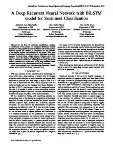
Fig. 1.

3

Overview of the proposed framework for point cloud classification.

component can contain more than one object. In the connected component, the local highest point may represent the top of the object. To further break the connected component into small pieces, a moving window algorithm is applied to search the local highest points. When the local highest points are found, the graph cut [57] is employed to segment the connected component, and the local highest points are taken as seeds. After the graph cut is performed, the connected component is divided into several point clusters. Each of the point clusters may still contain more than one object. Motivated by the fact that the normalized cut [58] can aggregate the points with uniform distribution into one cluster, it has been employed here to partition a large point cluster into two new clusters under the condition that the number of points in the cluster is larger than a predefined threshold, which is an over-segmentation process. In this way, we construct multilevel point clusters to capture from the coarse to fine parts of the objects. The size of each point cluster is determined by the point density and the object size. Here, three levels are used. Then we utilize [23] to construct the point-based feature descriptors. For each point, a feature vector with 18 dimensions, which contains the eigenvalue feature with six dimensions and the spin image feature with 12 dimensions, is computed through its k-nearest neighborhoods, where k = 30, 60, and 90, respectively. Thus, we obtain a 54-D feature vector for each point. Finally, the features of the points in a point cluster are aggregated into an n × 54 feature matrix, where n is the point number of the cluster. The feature matrix is taken as an input of the DNNSP. In the training process, the clusters of all levels are utilized to create a more discriminative feature representation. In the testing stage, we only classify the points in the clusters with the finest level. The aim is to reduce the probability that a cluster contains more than one class. The DNNSP should be invariant to the point permutation and sizes of the input point clusters. Therefore, a simple way for achieving this goal is to determine a point-based feature representation by the MLP and retain the weight sharing for each point, which means that the weight of each point in the same layer is the same. Then, max pooling is employed to aggregate the point-based features into the cluster-based features. Finally, the cluster-based features are put into another

MLP for point cloud classification. The basic architecture of our method for point cloud classification is shown in Fig. 1. In Fig. 1, the point-based feature representation processed by the MLP is illustrated by the yellow rectangle. The numbers in the brackets are the layer sizes of the MLPs. Based on the architectures, we will expand them in Section IV-B. B. Point-Based Feature Representations The spin images and eigenvalue feature descriptors describe different characteristics of a point. Since the intrarelations between the same type of feature descriptors is closer than the interrelations between different types of feature descriptors, the representations of the spin images and eigenvalue features are learned separately by the MLP. They are concatenated and further processed by another MLP to obtain the feature representations of each point in the point clusters. The process is shown in Fig. 2. C. Spatial Pooling In the point-based feature descriptors, we do not consider the spatial relationships among the points. To find spatial layout of the points, the DMst [20] is utilized to organize the points in each point cluster by taking the point nearest to the center of the point cluster as the root node. The DMst is a spanning tree, which combines the advantages of the minimum spanning tree (MST) and the spanning tree obtained by the Dijkstra algorithm. The MST can preserve the local structures. The Dijkstra algorithm solves the singlesource shortest path problem. The Dijkstra algorithm gives a good approximation of tree skeletons even if the point cloud is incomplete or noisy. Unfortunately, it cannot describe the spatial distribution of points in local regions. Since the DMst integrates the advantages of the above two types of trees, the leaf nodes and the nodes that connect with the leaf nodes in the DMst are usually the marginal points of a point cluster, because the marginal points are usually diffused and far away from the center of the cluster. The remaining nodes are the body points. Next, we separately handle the body points and marginal points in the DNNSP by configuring different weights for them in the feature representation. In this way, the cluster-based

This article has been accepted for inclusion in a future issue of this journal. Content is final as presented, with the exception of pagination. 4

Fig. 2.

IEEE TRANSACTIONS ON GEOSCIENCE AND REMOTE SENSING

Point-based feature representation process.

Fig. 3. Architecture of the DNNSP. RE stands for the eigenvalue feature descriptor. RSI denotes the spin image descriptor. RAF stands for the final point-based feature representation. (a) Architectures of the DNNSP. (b) Details in the red box of (a). (c) Details in the orange box of (a).

features contain two parts: one part arises from the marginal points and another arises from the body points. A spatial pooling layer is followed behind each layer in the MLP of the point-based feature representation. In this layer, the average pooling is operated to extract the feature representations of a point (i.e., a node in the DMst) and its connected points. It is noted that the DMst-based spatial pooling is operated on all points in each cluster. The connected points of a DMst node in the cluster can contain the marginal points and body points. Thus, the information of each node within the cluster can flow to the points that are connected to it. Fig. 3(a) shows the architecture of the DNNSP, and the details in the red and orange boxes are shown

in Fig. 3(b) and (c). To simplify the description, the network in one red box is called Net REF (Net for representing each type of feature) and the network in one orange box is called Net RAF (Net for representing all types of features). In addition, the weights of the same type of features in body points (or marginal points) are shared in each layer of the DNNSP. D. Implementation In the DNNSP, the activation function is the min[5, elu(x)]. The method in [2] is utilized for initialization, and batch normalization [60] is used before the activation. We apply stochastic gradient descent (SGD) to train the DNNSP with a

This article has been accepted for inclusion in a future issue of this journal. Content is final as presented, with the exception of pagination. WANG et al.: DNNSP FOR 3-D POINT CLOUD CLASSIFICATION

mini-batch size of 128. In SGD, a learning rate of 0.0001 and a momentum of 0.9 are used. In the following experiment, four Net REFs and one Net RAF are used in the DNNSP.

5

TABLE I N UMBER OF P OINTS IN S CENES I–III

IV. E XPERIMENTAL R ESULTS To evaluate the performance of the DNNSP, the DNNSP is employed to classify point clouds of six urban scenes. We also compare the DNNSP with the following four methods. The first method (method I) is the one described by Wang et al. [20]. This method employs a multiscale and hierarchical framework to classify point clouds of cluttered urban scenes. In this framework, the features of point clusters are constructed by employing the latent Dirichlet allocation (LDA) [61]. The second method (method II) is the one described in [23]. In this method, the point cloud is split into hierarchical clusters with different sizes. Then, LDA and sparse coding are jointly performed to extract and encode the shape features of the multilevel point clusters. The features at different levels are used to capture information on the shapes of objects of different sizes. The third method (method III) is the one described by Guo et al. [28]. In this method, each point is associated with a set of derived features using geometric, multireturn, and intensity information, and the features are selected using JointBoost to evaluate their correlations. The fourth method (method IV) is the one described by Li et al. [17]. In this method, a set of point-based descriptors for recognizing point clouds are constructed. The initial 3-D labeling of the categories is generated by utilizing a linear SVM classifier. These initial classification results are globally optimized by the multilabel graph-cut approach, and then are further refined automatically by a local optimization approach based upon the object-oriented decision tree. A. Experimental Data Sets The point clouds of six urban scenes are used in the experiment. Scenes I and II: The two scenes come from Tianjin, China. The point clouds contain buildings, trees, and a few cars. The point density is 20–30 points/m2 . The eaves extend outside the building roofs. Due to scattering, numerous noisy points occur around the eaves, which causes the eaves to be easily misclassified. Scene III: The point cloud is the Vaihingen data set [62] provided by the International Society for Photogrammetry and Remote Sensing, which are covered by 10 strips. The average strip overlap is 30%. The point cloud mainly contains four categories, i.e., roofs, facades, shrubs and trees, and low vegetation. The point density is uneven. The average strip overlap is 30%, and the median point density is 6.7 point/m2. The point density varies considerably over the entire block depending on the overlap. In the regions covered only by one strip, and the mean point density is 4 point/m2. The data sets of Scenes I–III are airborne laser scanning (ALS) point clouds, obtained by a Leica ALS50 system with

a mean flying height of 500 m above the ground and a 45° field of view. Scenes IV–VI: The data sets are the terrestrial laser scanning (TLS) point clouds provided by Eidgenössische Technische Hochschule Zurich, Zürich, Switzerland, [63]. The point density is uneven. The point clouds contain natural terrain, high vegetation, low vegetation, buildings, hard scape, scanning artifacts, and cars. The algorithm for obtaining the point-based feature descriptors and the point clusters runs on a computer with an Intel Core i7-4790 processor at 3.60 GHz and 8-GB RAM. It takes about 21, 15, 21, 224, 265, and 247 min for all the points in Scenes I–VI, respectively. After all the point-based feature descriptors and the point clusters are obtained, the DNNSP runs on a computer with a Titan X GPU. It takes about 3 h for each training data in Scenes I–III. To show the generalization ability of the DNNSP, Scene IV is used as the training data and Scenes V and VI are used as the testing data. Training time for Scene IV costs about 5 h. Only a few seconds are cost on testing all these scenes by using DNNSP. B. Classification Results on the ALS Point Clouds For Scenes I and II, the method in [23] is utilized to construct the feature descriptors and point clusters. We divide Scene III into training data and testing data. The point cloud is clustered into multilevel point clusters whose sizes are 60, 120, and 240. Table I lists the number of points in the training and testing data of Scenes I–III. Tables II and IV list the classification performance of three scenes. Figs. 4–6 illustrate the training data, testing data, and classification results of the three scenes. In Figs. 4 and 5, the green points are on the buildings; the blue points are on the trees, and the red points are on the cars. In Fig. 6, the navy blue points are on the roofs, the orange points are on the facades, the light blue points are on the low vegetation, and the green points are on the shrubs and trees. In Figs. 4(d), 5(d), and 6(d), the gray points are the correctly classified points. As shown in Figs. 4–6, most of the points are classified correctly, indicating that the DNNSP can learn good point cluster features. In Scenes I and II, only the blue blocks in Figs. 4(c) and 3(c) are misclassified. In the blue block of Fig. 4(c), because of the large amount of noise around the eaves, these points look like on the crown. In the blue

This article has been accepted for inclusion in a future issue of this journal. Content is final as presented, with the exception of pagination. 6

IEEE TRANSACTIONS ON GEOSCIENCE AND REMOTE SENSING

TABLE II C OMPARISONS OF THE C LASSIFICATION R ESULTS OF S CENES I–III IN T ERMS OF P RECISION /R ECALL /F1-M EASURE AND A CCURACY

Fig. 4. Scene I. (a) Training data. (b) Testing data. (c) Classification results. (d) Highlighted misclassified points. The green points are on the buildings. The blue points are on the trees. The red points are on the cars. The gray points are the correctly classified points in (d).

Fig. 5. Scene II. (a) Training data. (b) Testing data. (c) Classification results. (d) Highlighted misclassified points. The green points are on the buildings. The blue points are on the trees. The red points are on the cars. The gray points are the correctly classified points in (d).

block of Fig. 5(c), there is a line structure isolated from the building. The line structure maybe on an edge of an eave, and most of the points on it are misclassified. The classification accuracy of the cars is lower than those of the buildings and trees. The reason is that there are insufficient car points in the training data. This causes that the car features of the DNNSP are not well trained. In Fig. 6, it is observed that most of the misclassified points occur at the object borders, such as the roofs crowding with the trees or borders between the roofs and facades. In these cases, the neighboring points may be on objects of a different class, which causes the point-based features less discriminative. However, except the border points between the roofs and facades, most of the facade points have been recognized correctly. Since our method can learn more robust features than other methods, it achieves the highest F1-measure except the tree category in Scene II and the recall of the facades in Scene III. In the three scenes, it is noted that the F1-measure of the cars and facades by using our method areal are higher than

those by using other methods, indicating that our method is competitive for classifying the categories with a few points. In Scene III, many of the roof and facade points are misclassified using other methods. The reason is mainly that the roof points are confused with the low vegetation points, and the facade points are confused with the shrubs and trees points. However, the four categories are all classified better than other methods, which demonstrate that our method can distinguish the categories even though they look similar in shapes. C. Classification Results of the TLS Point Clouds For Scenes IV–VI, the point clouds are divided into multilevel clusters with the sizes of 100, 300, and 500. To show the generalization ability of our method, Scene IV is used as the training data, and the two other scenes are used as the testing data. One-third of the clusters that belong to the size of 500 are taken as the training data, and the point clouds

This article has been accepted for inclusion in a future issue of this journal. Content is final as presented, with the exception of pagination. WANG et al.: DNNSP FOR 3-D POINT CLOUD CLASSIFICATION

7

Fig. 6. Scene III. (a) Training data. (b) Testing data. (c) Classification results. (d) Highlighted misclassified points. The navy blue points are on the roofs. The orange points are on the facades. The light blue points are on the low vegetation. The green points are on the shrubs and trees. TABLE III N UMBER OF THE P OINTS IN S CENES IV–VI

in Scenes V and VI are taken as the testing data. Table III lists the number of points in Scenes IV–VI. Table IV lists the classification accuracy of Scenes V and VI. In Fig. 7, the light green points are on a natural terrain; the dark green points are on high vegetation; the bright green points are on low vegetation; the red points are on buildings; the purple points are on hard scape; the orange points are on the scanning artifacts; and the pink points are on cars. The classification results on Scenes V and VI are not as good as those of Scenes I–IV. In the two scenes, the shape features of some of the categories are easily confused, such as high vegetation and low vegetation, hard scape, and the other categories, especially for the hard scape, which is a class that is not taken as a special object. The hard scape contains rocks that mingle with cars, fences that mingle with vegetation, and steles that mingle with cars or buildings. Even worse, there are many hard scape points in Scene IV. To fit these points, the DNNSP is overfitting. All of the above reasons lead to the low classification accuracy for the hard scape. Most of the car and low vegetation points are classified into the hard scape. Although there are many car points, only three car samples are in Scene I. The training data of the cars are insufficient.

Fig. 7. Portion of the point clouds of Scenes IV–VI and training data and classification results of Scenes V and VI. (a) Point cloud in Scene IV. (b) Training data. (c) Point cloud in Scene V. (d) Classification results of (c). (e) Point cloud in Scene VI. (f) Classification results of (e). The light green points are on the natural terrain. The dark green points are on high vegetation. The bright green points are on low vegetation. The red points are on buildings. The purple points are on hard scape. The orange points are on the scanning artifacts. The pink points are on cars.

In addition, the cars are similar to rocks. Therefore, the performance of car classification is not good. The vegetation fences belong to low vegetation, but the fences made of other materials belong to hard scape. They are very similar in the point clouds; thus, the classification performance of the class fences is also not high. The high vegetation and low vegetation are also confused. The reason is that there are no clearly differences between them in terms of shapes. If the height is used, the performance will be improved. The natural terrain and buildings are classified correctly, which indicates that the accuracy is high if the sample size is sufficiently large. Compared with other methods, our method achieves the highest classification accuracy. The accuracy improves at least 20% for Scene VI. It means that the DNNSP has the ability to learn better feature representations from the point-based features and improve the classification accuracy. Moreover, the improvement is more obvious in complicated scenes. D. Performance of the Architectures in the DNNSP 1) Classification Performances of Net REF, Net RAF, and Spatial Pooling: Different numbers of Net REF and Net RAF are utilized to present the influences of the nets on the classification. Table V lists the classification accuracy (%) of Scenes I–VI through the DNNSP with 0–4 Net REF and 0–3 Net RAF,

This article has been accepted for inclusion in a future issue of this journal. Content is final as presented, with the exception of pagination. 8

IEEE TRANSACTIONS ON GEOSCIENCE AND REMOTE SENSING

TABLE IV

TABLE V

C OMPARISONS OF THE C LASSIFICATION R ESULTS OF S CENES V AND VI IN T ERMS OF P RECISION /R ECALL /F1-M EASURE AND A CCURACY

C LASSIFICATION A CCURACY (%) T HROUGH THE DNNSP W ITH /W ITHOUT S PATIAL P OOLING

with/without spatial pooling. The highest classification results are highlighted in bold. The poor classification results are replaced by “-.” As listed in Table V, for the classification results obtained by using at least one Net REF. It means that the use of intrarelations of the point-based features in the Net REF is helpful for improving the classification performance. One Net RAF is sufficient in the classification. In most cases, the more the Net RAFs are applied, the worse the classification results are. When the number of points increases in Scenes III, V, and VI, the Net RAF improves the classification performance. This indicates that the intrarelations of

the point-based features still have a little positive influence on the classification. In addition, simply concatenating the two types of features, i.e., spin images and eigenvalue features, into a vector is not a good idea. In the future work, we will find a better way to mine the interrelations. In Scenes I–III, sometimes the classification accuracy has a sudden decrease as the number of nets changes. This situation does not occur in Scenes V and VI. We argue that the points in Scenes I–III are few and the DNNSP can easily converge to a local minimum or overfitting. The DNNSP with spatial pooling achieves better classification results than does the DNNSP without spatial pooling, and it also enhances the classification performance of all of the scenes. When the number of Net RAFs is determined, the classification accuracy with spatial pooling is enhanced with an increase in the number of Net REFs, but the classification accuracy without spatial pooling is random. It is concluded that with the help of spatial pooling, the DNNSP can be stacked deeply to obtain better classification performance through more Net REFs. 2) Classification Results by Separating the Body and Margin Points: To show the advantages of separately using the body and margin points for the point cloud classification, we use all of the points without distinguishing the body points and margin points to classify the scenes. We observe from Table VI that the classification performance without distinguishing the body points and margin points is reduced

This article has been accepted for inclusion in a future issue of this journal. Content is final as presented, with the exception of pagination. WANG et al.: DNNSP FOR 3-D POINT CLOUD CLASSIFICATION

TABLE VI R ELATIVE I MPROVEMENTS BY U SING A LL OF THE P OINTS W ITHOUT D ISTINGUISHING THE B ODY P OINTS AND M ARGIN P OINTS

TABLE VII R ELATIVE I MPROVEMENTS BY U SING THE P OINT C LUSTERS W ITH O NE L EVEL

except in Scene II, especially for Scenes V and VI which are more complex. It demonstrates that distinguishing the body points and margin points can help to improve the classification accuracy of complex scenes. 3) Classification Results by Using All of the Levels of Clusters: To evaluate the effectiveness of the learned common features in the DNNSP, we take the point clusters with the smallest size as the input. The changes of classification results are listed in Table VII. From Table VII, it is observed that the classification accuracies are obviously lower than those obtained using all levels in Scenes I–III, which shows that the common features are helpful for the classification. V. C ONCLUSION The features learned by most of the current deep learning methods can obtain high-quality image classification results. However, many of these methods are hard to be applied to recognize 3-D point clouds due to unorganized distribution and various point density of data. In this paper, we have presented the DNNSP to classify outdoor point clouds without rasterization. The DMst-based pooling utilizes spatial information among points in the point clouds. The body points and marginal points in the DNNSP are handled separately by configuring different weights for them in the feature representation. In this way, the DNNSP can learn the feature representations of points from multiple levels, which makes the point clusterbased feature representations robust and discriminative. The experimental results have demonstrated the effectiveness of the DNNSP for point cloud classifications. By using the similar process with the input of PointNet [52] or using the recurrent neural network [55] that considers the point set as a sequential signal to learn point-based features, our framework can be seen as an end-to-end learning. In the future work, we will directly learn features from the raw point clouds, and extend our method into an end-to-end learning framework. R EFERENCES [1] C. Ma, X. Li, C. Notarnicola, S. Wang, and W. Wang, “Uncertainty quantification of soil moisture estimations based on a Bayesian probabilistic inversion,” IEEE Trans. Geosci. Remote Sens., vol. 55, no. 6, pp. 3194–3207, Jun. 2017. [2] X. Li et al., “Toward an improved data stewardship and service for environmental and ecological science data in West China,” Int. J. Digit. Earth, vol. 4, no. 4, pp. 347–359, Feb. 2011.

9

[3] Y. Liu and X. Li, “Domain adaptation for land use classification: A spatio-temporal knowledge reusing method,” ISPRS J. Photogramm. Remote Sens., vol. 98, pp. 133–144, Dec. 2014. [4] X. Xu, X. Li, X. Liu, H. Shen, and Q. Shi, “Multimodal registration of remotely sensed images based on Jeffrey’s divergence,” ISPRS J. Photogramm. Remote Sens., vol. 122, pp. 97–115, Dec. 2016. [5] B. Zhang, X. Sun, L. Gao, and L. Yang, “Endmember extraction of hyperspectral remote sensing images based on the ant colony optimization (ACO) algorithm,” IEEE Trans. Geosci. Remote Sens., vol. 49, no. 7, pp. 2635–2646, Jul. 2011. [6] B. Zhang, X. Sun, L. Gao, and L. Yang, “Endmember extraction of hyperspectral remote sensing images based on the discrete particle swarm optimization algorithm,” IEEE Trans. Geosci. Remote Sens., vol. 49, no. 11, pp. 4173–4176, Nov. 2011. [7] L. Yuan, Z. Yu, W. Luo, L. Yi, and G. Lü “Multidimensionalunified topological relations computation: A hierarchical geometric algebra-based approach,” Int. J. Geograph. Inf. Sci., vol. 28, no. 12, pp. 2435–2455, Jun. 2014. [8] L. Yuan, Z. Yu, W. Luo, Y. Hu, L. Feng, and A-X. Zhu, “A hierarchical tensor-based approach to compressing, updating and querying geospatial data,” IEEE Trans. Knowl. Data Eng., vol. 27, no. 2, pp. 312–325, Feb. 2015. [9] H. Hu, Q. Zhu, Z. Du, Y. Zhang, and Y. Ding, “Reliable spatial relationship constrained feature point matching of oblique aerial images,” Photogramm. Eng. Remote Sens., vol. 81, no. 1, pp. 49–58, Jan. 2015. [10] Q. Zhu, Y. Li, H. Hu, and B. Wu, “Robust point cloud classification based on multi-level semantic relationships for urban scenes,” ISPRS J. Photogram. Remote Sens., vol. 129, pp. 86–102, Jul. 2017. [11] S. Mei, M. He, Y. Zhang, Z. Wang, and D. Feng, “Improving spatial-spectral endmember extraction in the presence of anomalous ground objects,” IEEE Trans. Geosci. Remote Sens., vol. 49, no. 11, pp. 4210–4222, Nov. 2011. [12] S. Mei, M. He, Z. Wang, and D. Feng, “Spatial purity based endmember extraction for spectral mixture analysis,” IEEE Trans. Geosci. Remote Sens., vol. 48, no. 9, pp. 3434–3445, Sep. 2010. [13] D. Chen, L. Zhang, P. T. Mathiopoulos, and X. Huang, “A methodology for automated segmentation and reconstruction of urban 3-D buildings from ALS point clouds,” IEEE J. Sel. Topics Appl. Earth Observ. Remote Sens., vol. 7, no. 10, pp. 4199–4217, Oct. 2014. [14] D. Chen, R. Wang, and J. Peethambaran, “Topologically aware building rooftop reconstruction from airborne laser scanning point clouds,” IEEE Trans. Geosci. Remote Sens., vol. 55, no. 12, pp. 7032–7052, Dec. 2017. [15] B. Yang, Y. Zang, Z. Dong, and R. Huang, “An automated method to register airborne and terrestrial laser scanning point clouds,” ISPRS J. Photogram. Remote Sens., vol. 109, pp. 62–76, Nov. 2015. [16] A. Frome, D. Huber, R. Kolluri, T. Bülow, and J. Malik, “Recognizing objects in range data using regional point descriptors,” in Proc. Eur. Conf. Comput. Vis., May 2004, pp. 224–237. [17] Z. Li et al., “A three-step approach for TLS point cloud classification,” IEEE Trans. Geosci. Remote Sens., vol. 54, no. 9, pp. 5412–5424, Sep. 2016. [18] M. Weinmann, S. Urban, S. Hinz, B. Jutzi, and C. Mallet, “Distinctive 2D and 3D features for automated large-scale scene analysis in urban areas,” Comput. Graph., vol. 49, pp. 47–57, Jun. 2015. [19] J. Zhang, X. Lin, and X. Ning, “SVM-based classification of segmented airborne LiDAR point clouds in urban areas,” Remote Sens., vol. 5, pp. 3749–3775, Jul. 2013. [20] Z. Wang et al., “A multiscale and hierarchical feature extraction method for terrestrial laser scanning point cloud classification,” IEEE Trans. Geosci. Remote Sens., vol. 53, no. 5, pp. 2409–2425, May 2015. [21] X. Xiong, D. Munoz, J. A. Bagnell, and M. Hebert, “3-D scene analysis via sequenced predictions over points and regions,” in Proc. IEEE Int. Conf. Robot. Autom., May 2011, pp. 2609–2616. [22] B. Yang, Z. Dong, G. Zhao, and W. Dai, “Hierarchical extraction of urban objects from mobile laser scanning data,” ISPRS J. Photogram. Remote Sens., vol. 99, pp. 45–57, Jan. 2015. [23] Z. Zhang et al., “A multilevel point-cluster-based discriminative feature for ALS point cloud classification,” IEEE Trans. Geosci. Remote Sens., vol. 54, no. 6, pp. 3309–3321, Jun. 2016. [24] S. Xu, R. Wang, and H. Zheng, “Road curb extraction from mobile lidar point clouds,” IEEE Trans. Geosci. Remote Sens., vol. 55, no. 2, pp. 996–1009, Feb. 2017. [25] H. Zheng, R. Wang, and S. Xu, “Recognizing street lighting poles from mobile LiDAR data,” IEEE Trans. Geosci. Remote Sens., vol. 55, no. 1, pp. 407–420, Jan. 2017.

This article has been accepted for inclusion in a future issue of this journal. Content is final as presented, with the exception of pagination. 10

[26] Y. Bengio, A. Courville, and P. Vincent, “Representation learning: A review and new perspectives,” IEEE Trans. Pattern Anal. Mach. Intell., vol. 35, no. 8, pp. 1798–1828, Aug. 2013. [27] K. Fukano and H. Masuda, “Detection and classification of pole-like objects from mobile mapping data,” ISPRS Ann. Photogram., Remote Sens. Spatial Inf. Sci., vol. 2, pp. 57–64, Sep./Oct. 2015. [28] B. Guo, X. Huang, F. Zhang, and G. Sohn, “Classification of airborne laser scanning data using JointBoost,” ISPRS J. Photogramm. Remote Sens., vol. 100, pp. 71–83, Feb. 2015. [29] M. Kragh, R. N. Jørgensen, and H. Pedersen, “Object detection and terrain classification in agricultural fields using 3D LiDAR data,” in Proc. Int. Conf. Comput. Vis. Syst., 2015. pp. 188–197. [30] D. Maturana and S. Scherer, “3D convolutional neural networks for landing zone detection from LiDAR,” in Proc. IEEE Int. Conf. Robot. Autom., May 2015, pp. 3471–3478. [31] Z. Wu et al., “3D ShapeNets: A deep representation for volumetric shapes,” in Proc. IEEE Conf. Comput. Vis. Pattern Recognit., Jun. 2015, pp. 1912–1920. [32] Z. Zhu, X. Wang, S. Bai, C. Yao, and X. Bai, “Deep learning representation using autoencoder for 3D shape retrieval,” in Proc. Int. Conf. Secur., Pattern Anal., Cybern., Oct. 2014, pp. 279–284. [33] H. S. Koppula, A. Anand, T. Joachims, and A. Saxena, “Semantic labeling of 3D point clouds for indoor scenes,” in Proc. Adv. Neural Inf. Process. Syst., 2011, pp. 244–252. [34] A. Golovinskiy, V. G. Kim, and T. Funkhouser, “Shape-based recognition of 3D point clouds in urban environments,” in Proc. IEEE 12th Int. Conf. Comput. Vis., Sep./Oct. 2009, pp. 2154–2161. [35] A. E. Johnson and M. Hebert, “Using spin images for efficient object recognition in cluttered 3D scenes,” IEEE Trans. Pattern Anal. Mach. Intell., vol. 21, no. 5, pp. 433–449, May 1999. [36] S. Pu, M. Rutzinger, G. Vosselman, and S. O. Elberink, “Recognizing basic structures from mobile laser scanning data for road inventory studies,” ISPRS J. Photogram. Remote Sens., vol. 66, pp. S28–S39, Dec. 2011. [37] N. Chehata, L. Guo, and C. Mallet, “Airborne lidar feature selection for urban classification using random forests,” Int. Arch. Photogram., Remote Sens. Spatial Inf. Sci., vol. 38, pp. 207–212, Sep. 2009. [38] N. Brodu and D. Lague, “3D terrestrial lidar data classification of complex natural scenes using a multi-scale dimensionality criterion: Applications in geomorphology,” ISPRS J. Photogram. Remote Sens., vol. 68, pp. 121–134, Mar. 2012. [39] T. Hackel, J. D. Wegner, and K. Schindler, “Fast semantic segmentation of 3D point clouds with strongly varying density,” ISPRS Ann. Photogram. Remote Sens. Spatial Inf. Sci., vol. 3, pp. 177–184, Apr. 2016. [40] R. Zhang, S. A. Candra, K. Vetter, and A. Zakhor, “Sensor fusion for semantic segmentation of urban scenes,” in Proc. IEEE Int. Conf. Robot. Autom., May 2015, pp. 1850–1857. [41] J. Niemeyer, F. Rottensteiner, U. Soergel, and C. Heipke, “Hierarchical higher order CRF for the classification of airborne LiDAR point clouds in urban areas,” Int. Arch. Photogram., Remote Sens. Spatial Inf. Sci., pp. 12–19, Jun. 2016. [42] J. Xie, Y. Fang, F. Zhu, and E. Wong, “Deepshape: Deep learned shape descriptor for 3D shape matching and retrieval,” in Proc. IEEE Conf. Comput. Vis. Pattern Recognit., Jun. 2015, pp. 1275–1283. [43] A. Stuhlsatz, J. Lippel, and T. Zielke, “Feature extraction with deep neural networks by a generalized discriminant analysis,” IEEE Trans. Neural Netw. Learn. Syst., vol. 23, no. 4, pp. 596–608, Apr. 2012. [44] A. Krizhevsky, I. Sutskever, and G. E. Hinton, “ImageNet classification with deep convolutional neural networks,” in Proc. Adv. Neural Inf. Process. Syst., 2012, pp. 1097–1105. [45] C. Farabet, C. Couprie, L. Najman, and Y. LeCun, “Learning hierarchical features for scene labeling,” IEEE Trans. Pattern Anal. Mach. Intell., vol. 35, no. 8, pp. 1915–1929, Aug. 2013. [46] R. Socher, B. Huval, B. Bhat, C. D. Manning, and A. Y. Ng, “Convolutional-recursive deep learning for 3D object classification,” in Proc. Adv. Neural Inf. Process. Syst., 2012, pp. 656–664. [47] S. Song, F. Yu, A. Zeng. A. X. Chang, M. Savva, and T. Funkhouser. (2016). “Semantic scene completion from a single depth image.” [Online]. Available: https://arxiv.org/abs/1611.08974 [48] H. Guan, Y. Yu, Z. Ji, J. Li, and Q. Zhang, “Deep learning-based tree classification using mobile LiDAR data,” Remote Sens. Lett., vol. 6, no. 11, pp. 864–873, Sep. 2015. [49] D. Prokhorov, “A convolutional learning system for object classification in 3-D lidar data,” IEEE Trans. Neural Netw., vol. 21, no. 5, pp. 858–863, May 2010.

IEEE TRANSACTIONS ON GEOSCIENCE AND REMOTE SENSING

[50] D. Maturana and S. Scherer, “VoxNet: A 3D convolutional neural network for real-time object recognition,” in Proc. IEEE/RSJ Int. Conf. Intell. Robots Syst., Sep./Oct. 2015, pp. 922–928. [51] C. R. Qi, H. Su, M. Niebßner, A. Dai, M. Yan, and L. J. Guibas, “Volumetric and multi-view CNNs for object classification on 3D data,” in Proc. IEEE Conf. Comput. Vis. Pattern Recognit., Jun. 2016, pp. 5648–5656. [52] J. Huang and S. You, “Point cloud labeling using 3D convolutional neural network,” in Proc. 23rd Int. Conf. Pattern Recognit. Dec. 2016, pp. 2670–2675. [53] R. Q. Charles, H. Su, M. Kaichun, and L. J. Guibas, “PointNet: Deep learning on point sets for 3D classification and segmentation,” in Proc. IEEE Conf. Comput. Vis. Pattern Recognit., Jul. 2017, pp. 77–85. [54] C. R. Qi, L. Yi, H. Su, and L. J. Guibas, “PointNet++: Deep hierarchical feature learning on point sets in a metric space,” in Proc. Adv. Neural Inf. Process. Syst., 2017, pp. 5105–5114. [55] F. Liu et al., “3DCNN-DQN-RNN: A deep reinforcement learning framework for semantic parsing of large-scale 3D point clouds,” in Proc. IEEE Int. Conf. Comput. Vis., Oct. 2017, pp. 5679–5688. [56] D. Chen, L. Zhang, Z. Wang, and H. Deng, “A mathematical morphology-based multi-level filter of LiDAR data for generating DTMs,” Sci. China Inf. Sci., vol. 56, no. 10, pp. 1–14, 2013. [57] Y. Boykov, O. Veksler, and R. Zabih, “Fast approximate energy minimization via graph cuts,” IEEE Trans. Pattern Anal. Mach. Intell., vol. 23, no. 11, pp. 1222–1239, Nov. 2001. [58] J. Shi and J. Malik, “Normalized cuts and image segmentation,” IEEE Trans. Pattern Anal. Mach. Intell., vol. 22, no. 8, pp. 888–905, Aug. 2000. [59] K. He, X. Zhang, S. Ren, and J. Sun, “Delving deep into rectifiers: Surpassing human-level performance on imageNet classification,” in Proc. IEEE Int. Conf. Comput. Vis., Dec. 2015, pp. 1026–1034. [60] S. Ioffe and C. Szegedy. (2015). “Batch normalization: Accelerating deep network training by reducing internal covariate shift.” [Online]. Available: https://arxiv.org/abs/1502.03167 [61] D. M. Blei, A. Y. Ng, and M. I. Jordan, “Latent dirichlet allocation,” J. Mach. Learn. Res., vol. 3, pp. 993–1022, Jan. 2003. [62] J. Niemeyer, F. Rottensteiner, and U. Soergel, “Contextual classification of LiDAR data and building object detection in urban areas,” ISPRS J. Photogram. Remote Sens., vol. 87, pp. 152–165, Jan. 2014. [63] T. Hackel, N. Savinov, L. Ladicky, J. D. Wegner, K. Schindler, and M. Pollefeys, “Semantic3D.net: A new large-scale point cloud classification benchmark,” ISPRS Ann. Photogram., Remote Sens. Spatial Inf. Sci., vol. 1, pp. 91–98, Jun. 2017.

Zhen Wang received the Ph.D. degree in geographical information sciences from Beijing Normal University, Beijing, China, in 2015. He is currently a Lecturer with the China University of Geosciences, Beijing. His research interests include the application of light detection and ranging in remote sensing and remote sensing image processing.

Liqiang Zhang received the Ph.D. degree in geoinformatics from the Institute of Remote Sensing Applications, Chinese Academy of Sciences, Beijing, China, in 2004. He is currently a Professor with the Faculty of Geographical Science, Beijing Normal University, Beijing. His research interests include remote sensing image processing, 3-D urban reconstruction, and spatial object recognition.

This article has been accepted for inclusion in a future issue of this journal. Content is final as presented, with the exception of pagination. WANG et al.: DNNSP FOR 3-D POINT CLOUD CLASSIFICATION

11

Liang Zhang is currently pursuing the Ph.D. degree with the Faculty of Geographical Science, Beijing Normal University, Beijing, China. His research interests include remote sensing imagery processing and 3-D urban modeling.

Yibo Zheng is currently pursuing the bachelor’s degree with the Faculty of Geographical Science, Beijing Normal University, Beijing, China. Her research interests include remote sensing image processing and image-based classification.

Roujing Li received the bachelor’s degree in geographic information science from Capital Normal University, Beijing, China, in 2018. She is currently pursuing the master’s degree with the Faculty of Geographical Science, Beijing Normal University, Beijing. Her research interests include remote sensing image processing and 3-D point cloud registration.

Zidong Zhu is currently pursuing the bachelor’s degree with the Faculty of Geographical Science, Beijing Normal University, Beijing, China. His research interests include remote sensing image processing and image-based segmentation.