using Transformer and Graph Convolutional Network. Anonymous. Abstract. Patent landscaping is a method that is employed for searching related patents ...
A Deep Patent Landscaping Model using Transformer and Graph Convolutional Network Anonymous
Abstract Patent landscaping is a method that is employed for searching related patents during the process of a research and development (R&D) project. To avoid the risk of patent infringement and to follow the current trends of technology development, patent landscaping is a crucial task that needs to be conducted during the early stages of an R&D project. Generally, the process of patent landscaping requires several advanced resources and can be tedious. Furthermore, the patent landscaping process has to be repeated throughout the duration of an R&D project. Owing to such reasons, the demand for automated patent landscaping is gradually increasing. However, the shortage of well-defined benchmarking datasets and comparable models makes it difficult to find related research studies. In this paper, an automated patent landscaping model based on deep learning is proposed. The proposed model comprises a modified transformer structure for analyzing textual data present in patent documents and a graph convolutional network for analyzing patent metadata. Six patent landscaping benchmarking datasets, which were produced by the Korean patent attorney, are proposed for determining the resources required for comparing related research studies. Obtained results indicate that the proposed model with the proposed datasets can attain state-of-the-art performance, and mean classification accuracy of 98% can be achieved.
1
Introduction
A patent is a significant deliverable in research and development (R&D) projects. A patent protects an assignee’s legal rights and also represents current technology development trends. To study technological trends and seize potential infringement patents, majority of the R&D projects conduct the task of patent landscaping, which involves collecting and analyzing patent documents related to the projects. Generally, the task of patent landscaping is a human-centric, tedious, and expensive process [Trippe, 2015; Abood and Feltenberger, 2018]. Researchers and patent attorneys create keyword sets
for querying related patents in large patent databases, eliminate unrelated patent documents, and extract valid patents related to their project. The valid retrieved patents can be accordingly represented as a contour map by employing various visualization techniques [Yang et al., 2010; Wittenburg and Pekhteryev, 2015]. However, since the participants of the process have to be familiar with the scientific domain as well, they are costly . Furthermore, the patent landscaping task has to be repeated regularly during an ongoing project for searching newly published patents. In this paper, a semi-supervised deep learning model for patent landscaping is proposed. The proposed model eliminates repeated patent landscaping tasks after initially selecting patent keywords and valid patent documents by employing a classification model based on deep learning. Additionally, the proposed model incorporates a modified transformer structure [Vaswani et al., 2017] and graph convolutional network (GCN) [Kipf and Welling, 2016]. Since a patent document can contain several textual features and bibliometric data, a modified transformer structure was applied for processing textual data and a GCN was applied for processing bibliometric data fields constituted as network-based. To compare the performance of the proposed model with existing models, benchmarking datasets for patent landscaping were introduced. Generally, owing to issues such as high cost and data security, appropriate benchmarking datasets are not available. Such benchmarking datasets are generally created by human experts such as patent attorneys. Through the incorporation of six datasets generated through the Korea Intellecutral Property STrategy Agancey (KISTA), we aim to contribute research resources towards machine learning based patent landscaping research. Experimental results indicate that the proposed model with the incorporated datasets can attain state-of-the-art performance, and the average classification accuracy for each dataset can be improved by approximately over 15%.
2
Patent Landscaping
The entire process of patent landscaping is shown in Figure 1. Generally, when searching for patent documents, a keyword query is generated using various technological keywords. Because many assignees do not allow their patents to be discovered easily in the search to gain an advantage in the infringement issues that may arise, they tend to write patent titles
Topic Selection
Keyword Candidate Listing
Search Query Formulation
Valid Patent Selection
Patent Retrieval
Patent Landscape Report
Regularly repeated task Figure 1: The general process of patent landscaping
and abstracts very generically or omit technical details [Tseng et al., 2007]. To deal with this problem, researchers work on completing search queries with complicated words or key phrases to reinforce the search [Magdy and Jones, 2011]. For example, the following search query is created, as shown in the box below. (”underwater glider*” or ”underwater vehicle*” or ”underwater drone”) AND (emergency or urgency)) AND (hull or shape or body or drag or ”fluid force” or ”fluid power” or CFD or ”computational fluid dynamic*” or PMM or ”Plana Motion Mechanism” or design* or test or measure* or sensing or control* or overcome or obstacle or obstruction or ”wireless communitcat*” or ”satellite communitcat*” or ”command protocol” or battery or cell or power or launch or recovery or server or database or display*) The primary focus here is the regular repetition process going back to search query formulation from valid patent selection, as shown in Figure 1. Once the search formula is created, it is necessary to track the new patents published regularly using a similar search formula. Because the first valid patent selection is similar to creating a training dataset of supervised learning, it is one of the tasks that can solve repetitive tasks with text classification. For this reason, patent classification is one of the areas that have been studied steadily in the past decade [Sureka et al., 2009; Chen and Chiu, 2011; Lupu et al., 2013]. Relatively recent studies have challenged the International Patent Code (IPC) classification by using long short-term memory (LSTM) [Shalaby et al., 2018] and a text convolutional neural network (text-CNN) [Li et al., 2018]. Google has developed automated patent landscaping technology using a deep neural network [Abood and Feltenberger, 2018]. However, the biggest weakness of previous studies is the lack of a suitable benchmarking dataset. Unlike the purpose of actual patent landscaping, IPC classification studies predict a fittable IPC code for each patent, which is already granted to all patents by assignees and patent examiners. This is not a useful application for patent landscaping in the real world. In the case of Google’s work, heuristic algorithms are used to generate the training dataset by using technology keywords, such as ”Internet of Things”. Because the keywords and datasets are too general, there is uncertainty in applying the model to real-world R&D project handling specifics and detailed technology for patent landscaping. To the best of the authors’ knowledge, a fittable benchmarking dataset, generated by human experts for patent landscaping in the detailed
Dataset
Full name
ENDV NGUG
Ensuring Technology of Nighttime Driver Visibility Next Generation Technology of Underwater Glider Marine Plant Technology Using Augmented Reality Technology Technology for 1MW Dual Frequency System Technology for Micro Radar Rain Gauge Technology for Geostationary Orbit Complex Satellite
MPUART 1MWDFS MRRG GOCS
Table 1: Patent landscaping benchmarking dataset
technology field is not available yet.
3
Proposed Datasets for Patent Landscaping
3.1
Data sources
We provide a benchmarking dataset for patent landscaping based on the KISTA patent trends reports. Every year, the Korean Patent Office publishes more than 100 patent landscaping reports through KISTA1 . In particular, most reports are available to validate the results of the trends report by disclosing the valid patent list together with the patent search query2 . Currently, more than 2,500 reports are disclosed. The kinds of technology in the reports are specific, concrete, and sometimes include fusion characteristics. We have constructed datasets for the six technologies listed in Table 1.
3.2
Data acquisition
To ensure the reproducibility of building patent datasets, we have built the benchmarking datasets using Google BigQuery public datasets. Most of the patent data in the KISTA report are obtained by the required use of a search query of the local Korean patent database service WIPS. We first constructed a Python module that converts the WIPS query into a Google BigQuery service query, extracted the patent dataset from BigQuery, and marked the valid patents among the extracted patents. In the case of patent search, other datasets may be extracted depending on the type of publication date and database to be searched. Therefore, we excluded the queried patents published after the original publication date depicted in the report.
3.3
Dataset description
We built extracted patent datasets of six technological areas from Google BigQuery, and the number of patents in each dataset are given in Table 2. 1
http://biz.kista.re.kr/patentmap/ Most of the search queries were based on the WIPS (https://www.wipson.com) service, which is a local Korean patent 2
Dataset name ENDV NGUG MPUART 1MWDFS MRRG GOCS
# of patents
# of valid patents
4,420,806 8,011 1,470,065 1,774,999 2,068,828 295,194
618 243 468 1,507 286 1,139
Table 2: Summary of proposed datasets
4
Deep Patent Landscaping Model
4.1
Model overview
(a) Transformer structure
(b) GCN structure
Figure 3: Structures of Transformer and GCN layers
4.2
Figure 2: Architecture of the deep patent landscaping model
Our proposed deep patent landscaping model is composed of two parts: a transformer [Vaswani et al., 2017] and a graph convolutional network(GCN) [Kipf and Welling, 2016]. These parts generate embedding vectors from the features of a patent. The model contains a concatenation layer of the embedding vectors and stacked neural net layers to classify valid patents, as shown in Figure 2. A Patents, which is a scientific document, has metadata fields called bibliometric. They include International Patent Code (IPC), Cooperative Patent Classification (CPC), and citation with textual data such as abstracts and document titles. They possess characteristics that are represented by graph-based information. For example, citation information can be converted into a citation network that represents how one patent cites another patent [Yoon and Park, 2004]. IPC and CPC, which are technical classification codes for patents, are used as sources of graph information for co-occurrence matrix; this matrix represents whether patents have the same IPC code. To determine the patent features, we apply the transformer encoder to extract the embedding vectors for textual data, and the GCN structure to extract the embedding vectors for metadata. Finally, we use binary cross-entropy as a loss function for the binary classification model. database company.
Base features
A patent has different types features3 . We used five features of a patent: the abstract, IPC, CPC, USPC, and FamilyID. The abstract is the only textual feature used. The abstract is a brief but important descriptions of the invention. Although we examined other textual features such as title, claim, and full description, their performance was poor compared to the abstract. We believe that they are either too short or too long to represent the patent features. Among the metadata fields, we use IPC, CPC and USPC. They are types of technological classification codes devised by the patent management organizations. Because these codes are determined by the inventors and examiners directly, they are good means to represent the characteristics of a patent. We found that the accuracy is lower when we use citations with classification codes despite examining it. We use FamilyID as the feature matrix of GCN. It is a useful identification code that represents the collection of technological patents filed by the same applicant.
4.3
Computational structures of Transformer and GCN
Transformer The core of our model is the output of embedding through the transformer and GCN layers. First, we used only the encoder part of the transformer to learn the abstract data of the patent, as shown in Figure 3a. Similar to a transformer structure, we stacked the encoder layer six times. We also used multihead self-attention and scaled dot-product attention without the modification of a transformer encoder. We set the number of heads of multi-head self-attention at 8. We used the pretrained embedding vector from word2vec for the entire patent datasets as input. When we tokenized the abstract text, the tag [SEP] was inserted at the beginning, and the tag [CLS] was inserted at the end of the sentence. We set the sequence 3
https://bit.ly/2IvkMHf
length of 128, and the hidden size was 512. To concatenate the output of the transformer with the GCN embedding vectors, we adopted the squeeze technique from BERT [Devlin et al., 2018] and converted the matrix (sequence length, embedding size) to vector (embedding size) based on [CLS]. GCN One GCN structure stacks two GCN layers to produce an embedding vector for one metadata field, as shown in Figure 3b. The formula for GCN layer is given by Equation ( 1).
Figure 5: A preprocessed adjacency matrix
5 H
(l+1)
�
˜ − 12
=σ D
˜ − 21
A˜D
H
(l)
W
(l)
�
(1)
The GCN layer first constructs a preprocessed adjacency matrix for each metadata CPC, IPC, and USPC using the cooccurrence information in a patent. It then constructs a onehot vector for the occurrence of FamilyIDs for each metadata field and stacks the one-hot vectors N times to create a feature matrix, H (l) . As shown in Figure 4, N denotes the number of elements for each metadata field, and F denotes the number of FamilyIDs. Next, the following a layer-wise propagation rule is used as shown in Figure 4 with the calculations of dot-product.
Experiments
5.1
Dataset
We measured the performance of the proposed model for the classification of valid patents in the six KISTA datasets. We extracted 8,000-40,000 patent data for each dataset from Google BigQuery and created training and test sets with 8:2 in the entire patent dataset after downsampling the number total datasets. The dataset we proposed can be downloaded via the URLs provided in the following Table 3. Dataset name
Training set
Test set
URL
ENDV NGUG MPUART 1MWDFS MRRG GOCS
989 394 749 2412 458 1824
248 99 188 603 115 457
bit.ly/2Xk2goS bit.ly/2U2eyQz bit.ly/2U2e4Kf bit.ly/2GEQRKW bit.ly/2TYzQi4 bit.ly/2VdasVL
Table 3: Datasets for experiments
5.2 Figure 4: A layer-wise propagation rule for proposed GCN
˜ − 21 A˜D ˜ − 12 is a preprocessed adjacency In Equation 1, D matrix. A˜ denotes the sum of adjacency matrix and an identity matrix called self-connection matrix. An adjacency matrix is a binary matrix representing the co-occurrence relationship which exists between the elements of metadata and the classification codes of the same patent. If two CPC codes exists in the same patent, the value of the column representing relationship between two codes in binary matrix is 1. Degree ˜ is a diagonal matrix that adds the values in adjamatrix, D, cency matrix row by row, and its size is the same as that of the adjacency matrix. We used ReLU as an activation function σ, and the final output size of the GCN structure was 128. Using the GCN structure, we extracted useful features of the patent by learning the relationship between classification codes that occurred together. As the values of GCN embedding vectors were close to 0, we applied batch normalization [Ioffe and Szegedy, 2015] to the embedding vectors before concatenating them with other embedding vectors from the transformer structure.
Hyperparameter settings
We extracted embedding vectors from the transformer and GCN built on a separate learning process. In the transformer, six encoder layers were stacked, and the number of multihead attention was 8. The total learning epoch, the batch size, the optimizer, the learning rate and the epsilon were 20, 64, Adam Optimizer [Kingma and Ba, 2014], 0.0001, and 1e-8 respectively. We set the sequence length, which is the maximum length of the input sentence, to 128, and padded it to 0 if it was shorter than 128. As a result, 512-dimensional embedding vectors were extracted for each word. In GCN, two GCN layers were used, and the total learning epoch was 200. 128-dimensional embedding vectors were extracted for each metadata from the GCN, and an averaged of the extracted embedding vectors was taken. We used the early stopping technique to decrease the total time of the learning process.
5.3
Evaluation metric
We used the accuracy and f1 score, which are commonly used in binary classification problems, as an evaluation metric. Because the datasets are highly imbalanced data, we learned the model after reducing the number of patents, which is similar to the number of valid patents.
Dataset ENDV NGUG MPUART 1MWDFS MRRG GOCS
TRF+GCN Acc F1 0.9919 0.9848 0.9946 0.9900 1.00 0.9934
0.99 0.98 0.99 0.98 1.00 0.99
TRF Acc F1 0.9597 0.8687 0.9255 0.9121 0.9130 0.9015
0.96 0.87 0.93 0.91 0.91 0.90
GCN Acc F1 0.7258 0.6212 0.7527 0.7496 0.7696 0.7287
0.72 0.62 0.75 0.75 0.77 0.73
APL Acc F1 0.9435 0.7576 0.8511 0.9171 0.8435 0.8534
0.94 0.77 0.85 0.92 0.85 0.86
Table 4: Accuracy and F1 scores scores of baseline and proposed model
5.4
Overall results
We compared our proposed model (TRF+GCN in Table 4) with Google’s proposed Automated Patent Landscaping (APL [Abood and Feltenberger, 2018] in Table 4) model, which was a baseline. The results showed that the proposed model had the highest performance, over 98% accuracy, in all datasets, as shown in Table 4. In particular, the results showed that a performance improvement of the proposed model is more than 20% compared to using only the GCN structure with metadata. In addition, our model attained the average of a 10% improvement or more over Google’s APL model, which was a baseline model. We will investigate the following subjects empirically, with regard to the layers and features that affect patent landscaping model. • Which indicators of textual data and metadata have more influence on the model? • Which of the features, including citation information, has the most impact on the classification of patent landscaping? • When a misclassification occurs, what are the characteristics of the dataset that is misclassified?
5.5
Textual data vs. metadata represented in graph structure
In the first experiment, we found that a significant level of performance can be obtained only by textual data and abstract, that is compared with the data that can be represented as a graph and bibliometric data. This is because most of the datasets that we use are convergence technology, which cannot be distinguished only by the existing patent technology classifications. In other words, with the patent landscaping process, it is difficult to classify the technology type of the patents only by the patent technology classification code defined by the existing patent-related organizations such as United States patent and trademark office (USPTO) and World Intellectual Property Organization (WIPO). For example, an electric vehicle battery technology may not only include not only a device but also various technology groups such as an electric car battery material and a coolant. Therefore, by considering the contents of the patent along with the patent technology classification code, we can classify the patent according to the exact purpose. As shown in Table 4, we can found that there is a certain performance correlation
between the transformer only model and APL model. However, the GCN-only model has a relatively weak correlation. This also shows the difficulty in classifying a patent in R&D projects only with classification codes of the existing patents exclusively.
5.6
Classification codes vs. citation information
Our second question is, how effective is the presently and widely used citation information in patent landscaping? In conclusion, though citation information is as effective as the classification codes, it is more convenient to use only classification codes. As shown in table 6, 3CODE means that the model uses the transformer with the GCN including IPC, CPC, and United States Patent Classification System (USPC). REF means that the model uses the transformer with the GCN including citation information only. 4CODE means that the model uses the transformer with the GCN including all the metadata mentioned above. The performances of the 3CODE and REF are not significantly different, but in most cases, the performance of 3CODE is higher than that of the REF-only. In addition, when using 4CODE in a special case, the performance is lower than the case of using only the REF or 4CODE. We assume the reason is that the citation information can have several kinds of noise. In a patent citation, inventors cited not only the prior patent in the same application but also the patent related to the principle technology Sometimes, the principle technology patent is rare and not related to all the same technology application patents. In addition, technology classification codes have the advantage that the learning space is relatively small compared to the citation because the range that can be made in a similar patent field is narrowed. For this reason, technology classification codes are more fitting features than citation information in patent landscaping.
5.7
Which factors result in misclassification?
Our model achieved a performance improvement of 10% compared to the existing model and over 98% accuracy in the patent landscaping applicable to the proposed dataset. However, there are misclassifications. The following characteristics are consider as the reasons for the misclassifications. First, when the length of the abstract sequence is too long or short, the model does not perform well. We set the length of the abstract as 128 words, and force padding or truncating if the abstract is too long or short. When there is significant 0 padding of truncating, it seems misclassification may occur.
Dataset ENDV NGUG MPUART 1MWDFS MRRG GCOS
Metric
3CODE
CITATION
4CODE
Acc F1 Acc F1 Acc F1 Acc F1 Acc F1 Acc F1
0.9919 0.99 0.9848 0.98 0.9946 0.99 0.9900 0.98 1.00 1.00 0.9934 0.99
0.9879 0.98 0.9848 0.98 0.9893 0.93 0.9800 0.98 0.9739 0.97 0.9890 0.98
0.9919 0.99 0.9797 0.97 0.9760 0.75 0.9834 0.98 0.9826 0.98 0.9759 0.97
Table 5: Performance comparison between classification codes and citation information Dataset
true avg
true std
false avg
false std
ENDV NGUG MPUART 1MWDFS MRRG GOCS
109.72 104.63 110.05 106.46 107.7 121.34
43.94 40.72 42.15 44.77 42.31 45.98
128.12 123.86 109.26 106 125.6 122
50.51 45.77 29.02 42.17 27.46 45.03
Table 6: Length of the abstract
Second, in the case of misclassification category, the total average length of the abstract is about 110 and it is longer than that of well-classified data. Finally, since the numbers and special characters are removed during preprocessing, when there are many numbers or special characters in the abstract, the data are unable to express the information correctly, resulting in a drop in the classification. In the case of metadata, when only the abstract and classification codes are used, if the source of features is not sufficient, misclassification may occurs.
6
Conclusion and Future Work
In this paper, we proposed a deep patent landscaping model that solves the classification problem in patent landscaping using Transformer and GCN structures. This research suggested a new benchmarking dataset for the automated patent landscaping task and worked to make it a practical study for automated patent landscaping. In particular, it is anticipated that it will be possible to reduce the repetitive patent analysis tasks of practitioners performing patent analysis tasks. The main contributions of our research are as follows. • We released a new patent landscaping dataset that has been categorized by experts. • We propose a state of the art model which is at a level applicable to the real world. • We examined the features of a patent that can be used for patent landscaping. We discovered the following points about the use of patent features for automated patent landscaping. We need to consider both graphical information such as bibliometric as well
as textual data to achieve the highest classification performance. The classification codes specified by inventors in static metadata are available as a useful feature in patent landscaping. The combination of citation information and classification codes are not recommended. We think that we have developed a model for patent landscaping that have a possibility to be commercialized at a laboratory scale. In the future, we will build a system that can support to build benchmark datasets of over 2000 KISTA datasets to verify the scalability of the model. We will also build models that can classify not only US patents but also European, Japanese, Chinese and Korean patents. Particulary, Japanese patents are classified with additional code schemes, namely F-Term, which do not necessarily share similar characteristics with IPC and need further consideration. In the long term, our goal is to construct a fully automated classification system for patent landscaping that customized for the company and government organization.
References [Abood and Feltenberger, 2018] Aaron Abood and Dave Feltenberger. Automated patent landscaping. Artificial Intelligence and Law, 26(2):103–125, June 2018. [Chen and Chiu, 2011] Yen-Liang Chen and Yu-Ting Chiu. An ipc-based vector space model for patent retrieval. Information Processing & Management, 47(3):309–322, 2011. [Devlin et al., 2018] J. Devlin, M.-W. Chang, K. Lee, and K. Toutanova. BERT: Pre-training of Deep Bidirectional Transformers for Language Understanding. arXiv e-prints, October 2018. [Ioffe and Szegedy, 2015] Sergey Ioffe and Christian Szegedy. Batch normalization: Accelerating deep network training by reducing internal covariate shift. In International Conference on Machine Learning, pages 448–456, 2015. [Kingma and Ba, 2014] D. P. Kingma and J. Ba. Adam: A Method for Stochastic Optimization. arXiv e-prints, December 2014. [Kipf and Welling, 2016] Thomas N Kipf and Max Welling. Semi-supervised classification with graph convolutional networks. arXiv preprint arXiv:1609.02907, 2016. [Li et al., 2018] Shaobo Li, Jie Hu, Yuxin Cui, and Jianjun Hu. Deeppatent: patent classification with convolutional neural networks and word embedding. Scientometrics, 117(2):721–744, 2018. [Lupu et al., 2013] Mihai Lupu, Allan Hanbury, et al. Patent R in Information Reretrieval. Foundations and Trends trieval, 7(1):1–97, 2013. [Magdy and Jones, 2011] Walid Magdy and Gareth JF Jones. A study on query expansion methods for patent retrieval. In Proceedings of the 4th workshop on Patent information retrieval, pages 19–24. ACM, 2011. [Shalaby et al., 2018] Marawan Shalaby, Jan Stutzki, Matthias Schubert, and Stephan G¨unnemann. An lstm
approach to patent classification based on fixed hierarchy vectors. In Proceedings of the 2018 SIAM International Conference on Data Mining, pages 495–503. SIAM, 2018. [Sureka et al., 2009] Ashish Sureka, Pranav Prabhakar Mirajkar, Prasanna Nagesh Teli, Girish Agarwal, and Sumit Kumar Bose. Semantic based text classification of patent documents to a user-defined taxonomy. In International Conference on Advanced Data Mining and Applications, pages 644–651. Springer, 2009. [Trippe, 2015] Anthony Trippe. Guidelines for preparing patent landscape reports. Patent landscape reports. Geneva: WIPO, page 2015, 2015. [Tseng et al., 2007] Yuen-Hsien Tseng, Chi-Jen Lin, and YuI Lin. Text mining techniques for patent analysis. Information Processing & Management, 43(5):1216–1247, 2007. [Vaswani et al., 2017] Ashish Vaswani, Noam Shazeer, Niki Parmar, Jakob Uszkoreit, Llion Jones, Aidan N Gomez, Ł ukasz Kaiser, and Illia Polosukhin. Attention is all you need. In I. Guyon, U. V. Luxburg, S. Bengio, H. Wallach, R. Fergus, S. Vishwanathan, and R. Garnett, editors, Advances in Neural Information Processing Systems 30, pages 5998–6008. Curran Associates, Inc., 2017. [Wittenburg and Pekhteryev, 2015] K Wittenburg and G Pekhteryev. Multi-dimensional comparative visualization for patent landscaping. merl.com, 2015. [Yang et al., 2010] Y Y Yang, L Akers, C B Yang, T Klose, and S Pavlek. Enhancing patent landscape analysis with visualization output. 2010. [Yoon and Park, 2004] Byungun Yoon and Yongtae Park. A text-mining-based patent network: Analytical tool for high-technology trend. The Journal of High Technology Management Research, 15(1):37–50, 2004.