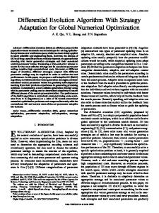
A Differential Evolution Algorithm Based on Individual ... - CiteSeerX

Journal of Computational Information Systems 8: 2 (2012) 717–725 Available at http://www.Jofcis.com

A Differential Evolution Algorithm Based on Individual-sorting and Individual-sampling Strategies Yang LOU 1 , Junli LI 1,2,∗, 1 Information 2 College

Gang LI 1

Science and Engineering College, Ningbo University, Ningbo 315211, China

of Computer Science, Sichuan Normal University, Chengdu 610066, China

Abstract In this paper we propose a novel hybrid version of Differential Evolution (DE). Firstly we modify the traditional structure of population in DE and propose a new strategy for population setting, in which the population is sorted in line with the fitness values of individuals. Another method is saltatory sampling with a nonrandom order, which is utilized to select candidates for the mutation operation. Furthermore, a strategy of survival of the fittest was used for individual selection operation. Combined the two strategies with DE, differential evolution based on individual-sorting and individual-sampling (ISSDE) is proposed, via testing on a series benchmark functions and compared with three variants of DE, the simulation results show that the proposed ISSDE has a better performance both in convergence speed and robustness. Keywords: Differential Evolution; Sorting; Sampling; Individual-sorting; Individual-sampling

1

Introduction

Evolutionary computation is a kind of problem solving system, which simulates the natural evolutionary process and provides foundation of computational intelligence [1]. The paradigm of evolutionary computing techniques dates back to early 1950s, when the idea to use Darwinian principles for automated problem solving originated and genetic algorithms (GAs) [2] has its origins in work done by biologists using computers to simulate natural genetic systems. Evolutionary programming (EP) [1] was introduced by Lawrence J. Fogel in the United States, while almost simultaneously, I. Rechenberg and H. P. Schwefel introduced evolution strategies (ESs) [1] in Europe. Research developments in Germany and the USA continued in parallel. These areas developed separately for about 15 years. Since the early 1990s, a fourth stream following the same general ideas started to emergegenetic programming (GP) [1]. Nowadays, the field of evolutionary computation includes GAs, EP, ESs, GP, differential evolution (DE) [3][4][5], as well as the swarm intelligence algorithms, for instance, ant colony optimization (ACO), particle swarm optimization (PSO), Bees algorithm, bacterial foraging optimization ∗

Corresponding author. Email address: [email protected] (Junli LI).

1553–9105 / Copyright © 2012 Binary Information Press January 2012

718

Y. Lou et al. /Journal of Computational Information Systems 8: 2 (2012) 717–725

(BFO) etc. The DE algorithm emerged as a very competitive form of evolutionary computing more than a decade ago, and was first proposed by R. Storn and K. Price in 1995. Later on many improved DE variants [6], such as improved SaDE, jDE, opposition-based DE (ODE), DE with global and local neighborhoods (DEGL), JADE and so on were proposed in the period 2006 to 2010 [6]. A series of DE variants based on sorting of individuals [7][8][9] are proposed, and the ordered structure of population enhances the performance of differential evolution a lot. DE as a special case of the GAs, has been proven able to solve a broad range of optimization problems, and thus has attracted even more attention in the last few years. DE is both robust and simple. In this paper, we proposed a novel variant of differential evolution algorithm ISSDE (individualsorting and individual-sampling based differential evolution), which based on two strategies named individual-sorting and individual-sampling, where the former reconstructs the structure of population and the later improves efficiency of selecting candidates in mutation. Owing to the details of mutation and selection are changed as well, such as strategy of survival of the fittest, ISSDE has remarkable advantages compared with its source version differential evolution.

2

Preliminaries

2.1

Problem definition

The purpose of global optimization is to find the optimal point / points for the objective function. Without loss of generality, we consider global minimization problems without constraint as optimization: Minimize f (x), subject to x ≤ x ≤ x, where point x = (x1 , x2 , · · · , xN ) is a variable vector in the search space RN , and f (·) is a single-objective function. Vectors x = (x1 , x2 , · · · , xN ) and x = (x1 , x2 , · · · , xN ) define the lower and upper boundaries of the variable x. The fitness value of a potential solution (a point in the search space) of the minimization problem is defined as −f (x).

2.2

Classic differential evolution description

An individual of differential evolution is biologically originated from the concept of chromosome, and are represented by vector x = (x1 , x2 , · · · , xN ). Individuals consist the population {xi , i = 1, 2, · · · , N P }, where N P represents the population size. The main operations of classic differential evolution algorithm can be summarized as follows: (1) M utation. A temporary individual vi is generated as: vi (g + 1) = xr1 (g) + F · (xr2 (g) − xr3 (g)), i 6= r1 6= r2 6= r3 where i, r1, r2, r3 ∈ [1, N P ], and r1, r2, r3 are randomly selected for each operation. Scale factor F > 0 is a real constant factor usually within range [0.5, 1]. (2) Crossover. The undetermined offspring ui is generated by crossover operation on vi and xi : ( vi,j (g + 1), if rand(0, 1) ≤ CR or j = jrand ui,j (g + 1) = vi,j (g), otherwise


719

where jrand is a randomly chosen index to ensure that the trail vector ui dose not duplicate xi . rand(0, 1) represents a uniform random value between 0 and 1, and CR ∈ (0, 1) is the crossover rate. (3) Selection. The better one of offspring and parent is selected into the next generation as follows: ( ui (g + 1), if f (ui (g + 1)) ≤ f (xi (g)) xi (g + 1) = xi (g), otherwise where, xi is the offspring of xi for the next generation.

2.3

Individual-sorting and sampling strategy

Individual-Sorting strategy was firstly proposed in ordering-binary differential evolution (OBDE) [7], which could generate several types of evolutionary algorithms, when it was combined with various mutation, crossover or selection operations. Among these operations, mutation makes the greatest effect. If an ergodic individual strategy is utilized in mutation, it is the ordering differential evolution (ODE) [8]. For ISSDE, candidates in mutation are selected from a sorted population, in which individuals’ qualities are clear to tell. Thus the better individuals sorted spearheaded, undertake the responsibility for generating good offspring and enhancing the precision of solutions as well, while the worse sorted in later sequence, take the responsibility for enhancing diversity of searching. An idea of considering both depth and width of searching is easy to realize in a sorted population. Especially in the later generations, individuals in consecutive order have tiny differences from each other. Therefore, we select an individual from several neighboring individuals as a representative of them. Exactly as we expected, individual-sampling strategy reduces the repetitive calculations a lot. Here neighboring indicates individuals with similar fitness values. The formular form of mutation strategy in ISSDE is a + F · (b − c), of which a was named the center-individual, while b and c were named second and last individual. A differential model of an eight-individual population is shown in Fig.1. According to the sorting 1 is the current best, which is the first center-individual in mutation, and principle, individual ○ the other two candidates are selected in the rests. For instance, we get V123 firstly, by individuals 1 ○ 2 and ○, 3 then ○ 1 and ○ 2 are hold on and the third candidate jump bN P/23 c = 1 (where bac ○, 4 thus, individuals ○, 1 ○ 2 and ○ 4 generate V124 , represents the maximal integer less than a) to ○, and then V125 · · · until the last individual participated. After the third candidate is completely sampled, the second candidate carries the same sequential sample, catching the progress above; 4 as the second candidate, then another. At last, bN P/21 c = 4 is it jumps bN P/22 c = 2 to ○ 5 becomes the center-individual in mutation. By parity of reasoning, the jumped, so individual ○ sorting-sample mutation strategy finishes the optimization. Note that second candidate should be chosen from individuals which are worse than the center-individual, and the third should be worse than the other two. Where 2i (i = 1, 2, 3) represents a sampling factor. Fig. 2 shows an example of ISSDE mutation, where offspring of x[i] is x[i]0 = x[i]±F (x[j]−x[k]), The location of the new individual should be quite near x[i], which has the best fitness value. The distance x[i] moves is determined by the absolute difference of x[j] and x[k], multiplying a random value, then the potential location of the offspring is at point A or B. On the evolutionary progress, good individuals have more opportunities than the bad to participate in mutation.

720


Fig. 1: Differential model of sorted population

3

Fig. 2: Illustration of mutation in ISSDE

Individual-sorting-sampling Based Differential Evolution

Fig. 3: ISSDE flow chart Fig.3 shows the flow chart of ISSDE, in the beginning of ISSDE, the initial population, i = 1, 2, · · · , N P are random initialized as: xi,j = xi,j + rand(0, 1) · (xi,j − xi,j ) where xi,j is the jth variable of the ith individual, the random number rand(0, 1) is uniformly distributed in interval (0, 1). According to the flow chart of ISSDE, a parameter ps is utilized to select using classic DE or ISSDE, where the value of rand is generated randomly. The operations of differential evolution


721

are introduced in previous section while the ISS (individual-sorting and individual-sampling) operation can be summarized as follows: (1) Sorting of Individuals. Individuals are evaluated and sorted by individuals’ fitnesses. {xi |i = 1, 2, · · · , N P } = {x1 , x2 , · · · , xN P |f (x1 ) ≤ f (x2 ) ≤ · · · ≤ f (xN P )} (2) Mutation. If |xm,j (g) − xn,j (g)| ≥ η, and |xn,j (g) − xl,j (g)| ≥ η, and |xm,j (g) − xl,j (g)| ≥ η, a temporary individual vtemp (g + 1) is generated: vtemp,j (g + 1) = xm,j (g) + F · |xn,j (g) − xl,j (g)|, m < n < l, F = sign · f · rand(0, 1) Otherwise, vtemp (g + 1) is randomly assigned: vtemp (g + 1) = xi,j + rand(0, 1) · (xi,j − xi,j ) where n ∈ [1, N P ], m ∈ [n + 1, N P ], l ∈ [m + 1, N P ]. sign is set as + or − with equal probability, and f is a constant that limits the range of scale factor F . η is a small value factor to ensure that the jth dimension (j = 1, 2, · · · D) of xm , xn and xl are not too closed. (3) Crossover. Two individuals including vtemp are involved in this operation to generate an offspring. ( vtemp,j (g + 1), if rand(0, 1) ≤ CR utemp,j (g + 1) = xrand,j (g), otherwise where CR ∈ [0, 1] is crossover rate, the subscript of xrand rand represents a random integers selected from the range of [1, N P ]. (4) Selection. The worst individual of parent generation is the comparative object of the newly generated individual, and the better one is retained in the next generation while the other is eliminated. ( utemp (g + 1), if f (utemp (g + 1)) ≤ f (xN P (g)) xN P (g + 1) = xN P (g), otherwise where xN P (g) has the worst fitness value of gth generation.

4

Convergence Proof

Individual-sorting and individual-sampling based differential evolution algorithm is a kind of randomized algorithms. The proving the convergence attribute of a randomized algorithm was firstly proposed by Solis and Wets [10]. They have given the theorems to prove whether an algorithm is converged to the global optimal in probability 1, which can be summarized as follows: Hypothesis. 1 [10] if f (D(z, ζ)) ≤ f (z), ζ ∈ S, then f (D(z, ζ)) ≤ f (ζ). Where D is the function to generate potential solutions, ζ is a random vector generated from the probability space (Rn , B, µk ), and f is the objective function. S is the subspace of Rn , represents

722


the constraint space of the problem. µk is probability measurement on B, which is the σ domain of Rn subset. Hypothesis. 2 [10] if A is a Borel subset of S, satisfied v(A) > 0, then ∞ Y

(1 − µk (A)) = 0

k=0

where v(A) a n-dimensional closure of subset A, and µk (A) is a probability, indicating the rate that µk generates A. Theorem.[10] Suppose f is a fathomable function, S is a fathomable subset of Rn , {zk }∞ 0 is a solution sequence generated by the randomized algorithm. If both Assumption 1 and Assumption 2 are satisfied simultaneously, then lim P [zk ∈ Rε ] = 1

k→∞

where Rε represents the set of the global optimal solutions. According to the theorem, if both Assumption 1 and Assumption 2 are satisfied simultaneously for ISSDE, it can be confirmed the proposed algorithm converges to the global optimal solution in probability 1. The convergence proof of ISSDE is given as follows: In the ISSDE algorithm, the return value before the iteration is the function value of xi (t − 1), i.e., f (xi (t − 1)) and f (xi (t)) represents the function value of the ith iteration value xi (t), where f (x) represents the objective function. The function D of Assumption 1 is defined as: ( D(xi (t − 1), xi (t)) =

xi (t − 1), if f (xi (t − 1)) ≤ f (xi (t)) xi (t),

if f (xi (t − 1)) > f (xi (t))

It can be inferred Assumption 1 is satisfied for ISSDE. For Assumption 2 all that is needed is to prove the S-sized sample space contains S, thus, S [

Mi,t ⊇ S

i=1

where Mi,t represents the support set of the individual’s sample space in ith iteration. Suppose there are N iterations in the search, and the range of the ith iteration is Si , which is the support set as well. Therefore, the union space of the population (a set of individuals) N S is Si . The range of an individual is adjustable, and when range covers the boundary of the i=1

solution space, though there are only a few individuals, it can as well enable S =

N S

Si Then

i=1

Assumption 2 is satisfied for ISSDE algorithm. In conclusion, ISSDE converges to the global optimal solution in probability 1, according to the theorem.


5 5.1

723

Experimental Studies Benchmark functions

(1) Sphere function: f1 =

D P

x2i , −5.12 ≤ xi ≤ 5.12, i = 1, 2, · · · , D, Minf1 = f1 (0, 0, · · · , 0) = 0

i=1 D P

(2) Rosenbrock function: f2 =

[100(xi+1 −x2i )2 +(xi −1)2 ], −5.12 ≤ xi ≤ 5.12, i = 1, 2, · · · , D,

i=1

Min f2 = f2 (1, 1, · · · , 1) = 0 (3) Rastrigin function:

D P

f3 =

(x2i − 10 cos(2πxi ) + 10), −5.12 ≤ xi ≤ 5.12, i = 1, 2, · · · , D,

i=1

Min f3 = f3 (0, 0, · · · , 0) = 0 (4) Ackley function:

r n n P 2 P f4 = 20 + e − 20 exp(−0.2 n1 zi ) − exp( n1 cos(2πzi )), −32 ≤ xi ≤ i=1

i=1

32, i = 1, 2, · · · , D, Min f4 = f4 (0, 0, · · · , 0) = 0 (5) Quartic function: f5 =

D P

[ix4i ], −2.56 ≤ xi ≤ 2.56, i = 1, 2, · · · , D, Min f4 = f4 (0, 0, · · · , 0)

i=1

=0

5.2

Comparison methods

The classic DE, ordering-binary differential evolution (OBDE) and ordering differential evolution (ODE) are used to evaluation the performance of ISSDE. The parameters DE are set as that proposed by Yang et al. [11], that is the population size N P = 30, crossover rate CR = 0.9, scale factor F = 0.5, and a mutation strategy of DE/rand/1.The population sizes of OBDE and ODE are set as DE above. The specific parameter of OBDE is constant C = 2, and both threshold factors of OBDE and ODE are η = 10−9 . The parameters of ISSDE are set as population size N P = 30, scale factor F = 1.5, crossover rate CR = 1.0, probability parameter Ps = 0.3, and threshold factor η = 10−9 . The halting condition is: 1. If the number of fitness function evaluations overstepped 2,000,000, then the running stopped; 2. Supposed Minf is the global optimum value, fbest is the current searched optimum value, if (|Minf − fbest | < ε(ε = 10−6 )), then the running stopped. Table I and II show the comparison of the results on 50-time independent random testing with the benchmark functions of 10-dimension. In Table I, Best/Worst indicates the best / worst solutions of the 50-time trails, and Std represents standard deviation, which indicates a divergence of the solutions. It is shown that DE and OBDE cannot always get the accurate solutions for f2, while ODE and ISSDE can. For other problems, all the algorithms can get solution within the accurate. In general, ODE gets the most accurate solutions, and both ODE and ISSDE get the standard deviations of e-7, which is corresponded to the halting conditions. In Table II, there listed the function evaluations (FEs) and succeed rate (SR) of the four algorithms on an average of 50-time independently trails. As it is corresponded to Table I, DE and OBDE cannot always get the accurate solutions for f2, particularly DE always cannot. OBDE is fastest algorithm for f3, while ISSDE is fastest in solving f1, f2, f4 and f5, which is directly

724


indicated from the function evaluations, the less the faster. In general, ISSDE is the fastest and the most rousts algorithm in solving the functions of 10-dimension. In consideration of solving higher dimensional problem, we test DE and ISSDE in the 30dimension function, considering OBDE and ODE are aiming at lower dimensional problems. In Table III, there listed the results of 50-time independent trails with 30-dimension benchmark functions. DE cannot get a accurate solution for f2, while ISSDE can get the accurate solutions for all functions. ISSDE needs much less function evaluations in general. It is worth noting that we set the population size 100 for DE [10], and keep the 30 population size for ISSDE. Table 1: Comparison of results on 50-time independent random testing with benchmark functions Test function

DE

D

OBDE

ODE

ISSDE

Best/Worst

Std

Best/Worst

Std

Best/Worst

Std

Best/Worst

Std

f1

1.45e-6/1.94e-6

e-7

1.096e-9/9.023e-7

e-7

1.42e-8/8.41e-7

e-7

7.44e-7/1.96e-6

e-7

f2

9.48e-2/1.91e-1

e-1

9.77e-7/1.51e-2

e-3

7.85e-7/9.98e-7

e-7

1.97e-6/1.99e-6

e-7

1.15e-6/1.93e-6

e-7

4.37e-11/9.88e-7

e-7

3.02e-11/6.83e-7

e-7

2.42e-8/1.99e-6

e-7

f4

1.33e-6/1.97e-6

e-7

7.46e-8/2.91e-5

e-6

1.45e-7/9.70e-7

e-7

1.19e-6/1.99e-6

e-7

f5

5.63e-7/1.96e-6

e-7

4.88e-11/-9.91e-7

e-7

1.08e-9/5.01e-7

e-7

1.82e-7/1.95e-6

e-7

10

f3

Table 2: Comparison of efficiency on 50-time independent random testing with benchmark functions Test function

DE

D

OBDE

FEs

SR

f1

17 636

50/50

8 451

f2

2 000 000

0/50

1 417 695

71 872

50/50

16 821

f4

36 744

50/50

f5

8 436

50/50

10

f3

FEs

ODE SR

ISSDE

FEs

SR

FEs

SR

50/50

17 406

46/50

464 656

50/50

2354

50/50

50/50

102 946

50/50

50/50

464 656

50/50

130 687

103 420

50/50

50/50

36 082

50/50

6048

4 797

50/50

50/50

8 312

50/50

1184

50/50

Table 3: Comparison of results on 50-time independent random testing with benchmark functions Test function D

ISSDE

Std

FEs

SR

Best/Worst

Std

FEs

SR

1.28e-6/1.96e-6

e-7

299 052

50/50

1.51e-6/1.99e-6

e-7

13 280

50/50

1.39e+2/1.69e+2

e+0

2 000 000

0/50

1.97e-6/1.99e-6

e-8

717 326

50/50

1.49e-6/1.99e-6

e-7

1 144 284

50/50

2.13e-7/1.98e-6

e-7

148 762

50/50

f4

1.74e-6/1.99e-6

e-8

591 036

50/50

1.63e-6/1.99e-6

e-8

114 671

50/50

f5

4.31e-7/1.98e-6

e-7

188 376

50/50

1.04e-6/1.99e-6

e-7

8 472

50/50

f1 f2 f3

6

DE (NP =100) Best/Worst

30

Conclusion

In this paper, we proposed a novel differential evolution algorithm named ISSDE, which is based on individual-sorting and individual-sampling, two important strategies to enhance the performance of differential evolution. A group of exploratory experiments were carried out to obtain good control parameters experimentally. The proposed ISSDE was compared with the DE, OBDE, and ODE by testing them on benchmark functions. The simulation results showed that ISSDE outperformed DE, OBDE, and ODE algorithms and the two used simple strategies improve the algorithm’s performance effectively.


725

Acknowledgement This research was supported by the Natural Science Foundation of Zhejiang Province under Grant No. Y1100076, K. C. Wong Magna Fund in Ningbo University, and the Scientific Research Foundation of Graduate School of Ningbo University.

References [1]

R. C. Eberhart and Y. H. Shi, Computational Intelligence: Concepts to Implementations. Elsevier, Singapore, 2009.

[2]

J. H. Holland. Adaptation in Natural and Artificial Systems. University of Michigan Press, Ann Arbor, 1975.

[3]

R. Storn and K. Price. Differential Evolution — A Simple and Efficient Heuristic for Global Optimization over Continuous Spaces. Journal of Global Optimization, vol. 11, pages 341 – 359, 1997.

[4]

R. Storn and K. Price. Differential Evolution — A simple and efficient adaptive scheme for global optimization over continuous spaces. Technical Report TR-95-012, ICSI, http://http.icsi.berkeley.edu/-storn/litera.html.

[5]

R. Storn. On the Usage of Differential Evolution for Function Optimization. In Proceedings of the Biennial Conference of the North American on Fuzzy Information Processing Society. USA. pages 519 – 523, 1996.

[6]

S. Das and P. N. Suganthan. Differential Evolution: A Survey of the State-of-the-Art. IEEE Transactions on Evolutionary Computation. 15 (1): 4 – 31, 2011.

[7]

Y. Lou, J. L. Li and Y. S. Wang. A Binary-Differential Evolution algorithm based on Ordering of individuals. In Proceedings the Sixth International Conference on Natural Computation (ICNC 10). China. vol. 5, pages 2207 – 2211, 2010.

[8]

Y. Lou, J. L. Li. A Differential Evolution algorithm based on Ordering of individuals. In Proceedings the 2nd International Conference on Industrial Mechatronics and Automation (ICIMA 10), China. vol. 2, pages 105 – 108, 2010.

[9]

Y. Lou, J. L. Li and Y. H. Shi, A Differential Evolution Based on Individual-Sorting and IndividualSampling Strategies. In Proceedings of the 2011 IEEE Symposium on Differential Evolution, France, pages 33 – 40, 2011.

[10] F. J. Solis and R. T. Wets. Minimization by Random Search Techniques. Mathematics of Operations Research. 6 (1): 19 – 30, 1981. [11] Z. Y. Yang, K. Tang and X. Yao. Self-adaptive Differential Evolution with Neighborhood Search. In Proceedings the 2008 IEEE Congress on Evolutionary Computation (CEC 08), pages 1110 – 1116, 2008.