A discriminative language model with pseudo-negative samples

A Discriminative Language Model with Pseudo-Negative Samples Daisuke Okanohara Jun’ichi Tsujii
 Department of Computer Science, University of Tokyo Hongo 7-3-1, Bunkyo-ku, Tokyo, Japan
School of Informatics, University of Manchester NaCTeM (National Center for Text Mining) hillbig,tsujii@is.s.u-tokyo.ac.jp

Abstract In this paper, we propose a novel discriminative language model, which can be applied quite generally. Compared to the well known N-gram language models, discriminative language models can achieve more accurate discrimination because they can employ overlapping features and nonlocal information. However, discriminative language models have been used only for re-ranking in specific applications because negative examples are not available. We propose sampling pseudo-negative examples taken from probabilistic language models. However, this approach requires prohibitive computational cost if we are dealing with quite a few features and training samples. We tackle the problem by estimating the latent information in sentences using a semiMarkov class model, and then extracting features from them. We also use an online margin-based algorithm with efficient kernel computation. Experimental results show that pseudo-negative examples can be treated as real negative examples and our model can classify these sentences correctly.

1 Introduction Language models (LMs) are fundamental tools for many applications, such as speech recognition, machine translation and spelling correction. The goal of LMs is to determine whether a sentence is correct or incorrect in terms of grammars and pragmatics. 73

The most widely used LM is a probabilistic language model (PLM), which assigns a probability to a sentence or a word sequence. In particular, Ngrams with maximum likelihood estimation (NLMs) are often used. Although NLMs are simple, they are effective for many applications. However, NLMs cannot determine correctness of a sentence independently because the probability depends on the length of the sentence and the global frequencies of each word in it. For example,




, where

is the probability of a sentence
given by an NLM, does not always mean that

is more correct, but instead could occur when

is shorter than
, or if

has more common words than
. Another problem is that NLMs cannot handle overlapping information or non-local information easily, which is important for more accurate sentence classification. For example, a NLM could assign a high probability to a sentence even if it does not have a verb. Discriminative language models (DLMs) have been proposed to classify sentences directly as correct or incorrect (Gao et al., 2005; Roark et al., 2007), and these models can handle both non-local and overlapping information. However DLMs in previous studies have been restricted to specific applications. Therefore the model cannot be used for other applications. If we had negative examples available, the models could be trained directly by discriminating between correct and incorrect sentences. In this paper, we propose a generic DLM, which can be used not only for specific applications, but also more generally, similar to PLMs. To achieve

Proceedings of the 45th Annual Meeting of the Association of Computational Linguistics, pages 73–80, c Prague, Czech Republic, June 2007. 2007 Association for Computational Linguistics

this goal, we need to solve two problems. The first is that since we cannot obtain negative examples (incorrect sentences), we need to generate them. The second is the prohibitive computational cost because the number of features and examples is very large. In previous studies this problem did not arise because the amount of training data was limited and they did not use a combination of features, and thus the computational cost was negligible. To solve the first problem, we propose sampling incorrect sentences taken from a PLM and then training a model to discriminate between correct and incorrect sentences. We call these examples PseudoNegative because they are not actually negative sentences. We call this method DLM-PN (DLM with Pseudo-Negative samples). To deal with the second problem, we employ an online margin-based learning algorithm with fast kernel computation. This enables us to employ combinations of features, which are important for discrimination between correct and incorrect sentences. We also estimate the latent information in sentences by using a semi-Markov class model to extract features. Although there are substantially fewer latent features than explicit features such as words or phrases, latent features contain essential information for sentence classification. Experimental results show that these pseudonegative samples can be treated as incorrect examples, and that DLM-PN can learn to correctly discriminate between correct and incorrect sentences and can therefore classify these sentences correctly.

2 Previous work Probabilistic language models (PLMs) estimate the probability of word strings or sentences. Among these models, N-gram language models (NLMs) are widely used. NLMs approximate the probability by  words. conditioning only on the preceding  For example, let
denote a sentence of  words,
   
      . Then, by the chain rule of probability and the approximation, we have







   
     


 

 









     





(1)

The parameters can be estimated using the maximum likelihood method. 74

Since the number of parameters in NLM is still large, several smoothing methods are used (Chen and Goodman, 1998) to produce more accurate probabilities, and to assign nonzero probabilities to any word string. However, since the probabilities in NLMs depend on the length of the sentence, two sentences of different length cannot be compared directly. Recently, Whole Sentence Maximum Entropy Models (Rosenfeld et al., 2001) (WSMEs) have been introduced. They assign a probability to each sentence using a maximum entropy model. Although WSMEs can encode all features of a sentence including non-local ones, they are only slightly superior to NLMs, in that they have the disadvantage of being computationally expensive, and not all relevant features can be included. A discriminative language model (DLM) assigns a score

to a sentence
, measuring the correctness of a sentence in terms of grammar and pragmatics, so that

 implies
is correct and

  implies
is incorrect. A PLM can be considered as a special case of a DLM by defining using 

. For example, we can take

 




, where is some threshold, and


is the length of
. Given a sentence
, we extract a feature vector (

) from it using a pre-defined set of feature functions      . The form of the function we use is

 

 (2)

Û

Û

where is a feature weighting vector. Since there is no restriction in designing

, DLMs can make use of both over-lapping and nonlocal information in
. We estimate using training samples 

 

 for   , where 
  if

is correct and 
  if

is incorrect. However, it is hard to obtain incorrect sentences because only correct sentences are available from the corpus. This problem was not an issue for previous studies because they were concerned with specific applications and therefore were able to obtain real negative examples easily. For example, Roark (2007) proposed a discriminative language model, in which a model is trained so that a correct sentence should have higher score than others. The difference between their approach and ours is that we do not assume just one application. Moreover, they had

Û

For i=1,2,... Choose a word 
at random according to the distribution  


       

If 
 "end of a sentence" Break End End

We know of no program, and animated discussions about prospects for trade barriers or regulations on the rules of the game as a whole, and elements of decoration of this peanut-shaped to priorities tasks across both target countries

Figure 2: Example of a sentence sampled by PLMs (Trigram).

Figure 1: Sample procedure for pseudo-negative examples taken from N-gram language models. training sets consisting of one correct sentence and many incorrect sentences, which were very similar because they were generated by the same input. Our framework does not assume any such training sets, and we treat correct or incorrect examples independently in training.

Build a probabilistic language model Probabilistic LM (e.g. N-gram LM) Sample sentences

Corpus Positive

(Pseudo-) Negative Input training examples

Binary Classifier

3 Discriminative Language Model with Pseudo-Negative samples We propose a novel discriminative language model; a Discriminative Language Model with PseudoNegative samples (DLM-PN). In this model, pseudo-negative examples, which are all assumed to be incorrect, are sampled from PLMs. First a PLM is built using training data and then examples, which are almost all negative, are sampled independently from PLMs. DLMs are trained using correct sentences from a corpus and negative examples from a Pseudo-Negative generator. An advantage of sampling is that as many negative examples can be collected as correct ones, and a distinction can be clearly made between truly correct sentences and incorrect sentences, even though the latter might be correct in a local sense. For sampling, any PLMs can be used as long as the model supports a sentence sampling procedure. In this research we used NLMs with interpolated smoothing because such models support efficient sentence sampling. Figure 1 describes the sampling procedure and figure 2 shows an example of a pseudo-negative sentence. Since the focus is on discriminating between correct sentences from a corpus and incorrect sentences sampled from the NLM, DLM-PN may not able to classify incorrect sentences that are not generated from the NLM. However, this does not result in a se75

test sentences Return positive/negative label or score (margin)

Figure 3: Framework of our classification process. rious problem, because these sentences, if they exist, can be filtered out by NLMs.

4 Online margin-based learning with fast kernel computation The DLM-PN can be trained by using any binary classification learning methods. However, since the number of training examples is very large, batch training has suffered from prohibitively large computational cost in terms of time and memory. Therefore we make use of an online learning algorithm proposed by (Crammer et al., 2006), which has a much smaller computational cost. We follow the definition in (Crammer et al., 2006). is initialized to and for The initiation vector each round the algorithm observes a training example



and predicts its label 

to be either  or . After the prediction is made, the true label 
is revealed and the algorithm suffers an instantaneous hinge-loss  
 


  



which reflects the degree to which its prediction was wrong. If the prediction was wrong, the parameter

Û

¼

Ü

Û Ü

Û Ü

Û is updated as Û



Û Û


  subject to  Û Ü  

  and   




Û














(3) (4)

where  is a slack term and  is a positive parameter which controls the influence of the slack term on the objective function. A large value of  will result in a more aggressive update step. This has a closed form solution as

Û




Û




 



Ü

(5)




where 
  Ü ¾ . As in SVMs, a final weight vector can be represented as a kerneldependent combination of the stored training examples.   


  (6)

Û Ü




Ü Ü




Using this formulation the inner product can be replaced with a general Mercer kernel 

such as a polynomial kernel or a Gaussian kernel. The combination of features, which can capture correlation information, is important in DLMs. If the kernel-trick (Taylor and Cristianini, 2004) is applied to online margin-based learning, a subset of the observed examples, called the active set, needs to be stored. However in contrast to the support set in SVMs, an example is added to the active set every time the online algorithm makes a prediction mistake or when its confidence in a prediction is inadequately low. Therefore the active set can increase in size significantly and thus the total computational cost becomes proportional to the square of the number of training examples. Since the number of training examples is very large, the computational cost is prohibitive even if we apply the kernel trick. The calculation of the inner product between two examples can be done by intersection of the activated features in each example. This is similar to a merge sort and can be executed in  
time where  is the average number of activated features in an example. When the number of examples in the active set is , the total computational cost is    
. For fast kernel computation, the Polynomial Kernel Inverted method (PKI)) is proposed (Kudo and Matsumoto, 2003), which is an extension of Inverted Index in Information Retrieval. This 76

ÜÜ

algorithm uses a table 

for each feature item, which stores examples where a feature
is fired. Let  be the average of



over all feature item. Then the kernel computation can be performed in    
time which is much less than the normal kernel computation time when  . We can easily extend this algorithm into the online setting by updating 

when an observed example is added to an active set.

5 Latent features by semi-Markov class model Another problem for DLMs is that the number of features becomes very large, because all possible Ngrams are used as features. In particular, the memory requirement becomes a serious problem because quite a few active sets with many features have to be stored, not only at training time, but also at classification time. One way to deal with this is to filter out low-confidence features, but it is difficult to decide which features are important in online learning. For this reason we cluster similar N-grams using a semi-Markov class model. The class model was originally proposed by (Martin et al., 1998). In the class model, deterministic word-to-class mappings are estimated, keeping the number of classes much smaller than the number of distinct words. A semi-Markov class model (SMCM) is an extended version of the class model, a part of which was proposed by (Deligne and BIMBOT, 1995). In SMCM, a word sequence is partitioned into a variable-length sequence of chunks and then chunks are clustered into classes (Figure 4). How a chunk is clustered depends on which chunks are adjacent to it. The probability of a sentence        
, in a bi-gram class model is calculated by

 



 





(7)




On the other hand, the probabilities in a bi-gram semi-Markov class model are calculated by




 









 
 


 







(8)




where varies over all possible partitions of
,  
and ! 
denote the start and end positions respectively of the -th chunk in partition , and    


! 
  for all . Note that each word or variablelength chunk belongs to only one class, in contrast to a hidden Markov model where each word can belong to several classes. Using a training corpus, the mapping is estimated by maximum likelihood estimation. The log likelihood of the training corpus (       ) in a bigram class model can be calculated as 






 










 

(9)





 



(10)






"   



½ ¾



"   

" 
" 



(11)

" 
 " 




where " 
, " 
and "   

are frequencies of a word , a class  and a class bi-gram   
in the training corpus. In (11) only the first term is used, since the second term does not depend on the class allocation. The class allocation problem is solved by an exchange algorithm as follows. First, all words are assigned to a randomly determined class. Next, for each word , we move it to the class  for which the log-likelihood is maximized. This procedure is continued until the log-likelihood converges to a local maximum. A naive implementation of the clustering algorithm scales quadratically to the number of classes, since each time a word is moved between classes, all class bi-gram counts are potentially affected. However, by considering only those counts that actually change, the algorithm can be made to scale somewhere between linearly and quadratically to the number of classes (Martin et al., 1998). In SMCM, partitions of each sentence are also determined. We used a Viterbi decoding (Deligne and BIMBOT, 1995) for the partition. We applied the exchange algorithm and the Viterbi decoding alternately until the log-likelihood converged to the local maximum. Since the number of chunks is very large, for example, in our experiments we used about  million chunks, the computational cost is still large. We therefore employed the following two techniques. The first was to approximate the computation in the exchange algorithm; the second was to make use of 77

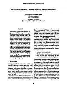
w1 w2 w3 w4 w5 w6 w7 w8 c1

c2

c3

c4

Figure 4: Example of assignment in semi-Markov class model. A sentence is partitioned into variablelength chunks and each chunk is assigned a unique class number. bottom-up clustering to strengthen the convergence. In each step in the exchange algorithm, the approximate value of the change of the log-likelihood was examined, and the exchange algorithm applied only if the approximate value was larger than a predefined threshold. The second technique was to reduce memory requirements. Since the matrices used in the exchange algorithm could become very large, we clustered chunks into  classes and then again we clustered these two into  each, thus obtaining  classes. This procedure was applied recursively until the number of classes reached a pre-defined number.

6 Experiments 6.1

Experimental Setup

We partitioned a BNC-corpus into model-train, DLM-train-positive, and DLM-test-positive sets. The numbers of sentences in model-train, DLMtrain-positive and DLM-test-positive were k, k, and k respectively. An NLM was built using model-train and Pseudo-Negative examples (k sentences) were sampled from it. We mixed sentences from DLM-train-positive and the PseudoNegative examples and then shuffled the order of these sentences to make DLM-train. We also constructed DLM-test by mixing DLM-test-positive and k new (not already used) sentences from the Pseudo-Negative examples. We call the sentences from DLM-train-positive “positive” examples and the sentences from the Pseudo-Negative examples “negative” examples in the following. From these sentences the ones with less than  words were excluded beforehand because it was difficult to decide whether these sentences were correct or not (e.g.

Accuracy (%) Training time (s) Linear classifier word tri-gram 51.28 137.1 POS tri-gram 52.64 85.0 SMCM bi-gram (#  ) 51.79 304.9 SMCM bi-gram (#  ) 54.45 422.1 rd order Polynomial Kernel word tri-gram 73.65 20143.7 POS tri-gram 66.58 29622.9 SMCM bi-gram (#  ) 67.11 37181.6 SMCM bi-gram (#  ) 74.11 34474.7 Table 1: Performance on the evaluation data. compound words). Let # be the number of classes in SMCMs. Two SMCMs, one with #   and the other with #  , were constructed from model-train. Each SMCM contained  million extracted chunks.

(Miyao and Tsujii, 2005). All sentences were parsed correctly except for one positive example. This result indicates that correct sentences and pseudonegative examples cannot be differentiated syntactically.

6.2

6.3

Experiments on Pseudo-Examples

We examined the property of a sentence being Pseudo-Negative, in order to justify our framework. A native English speaker and two non-native English speaker were asked to assign correct/incorrect labels to  sentences in DLM-train1 . The result for an native English speaker was that all positive sentences were labeled as correct and all negative sentences except for one were labeled as incorrect. On the other hand, the results for non-native English speakers are 67 and 70. From this result, we can say that the sampling method was able to generate incorrect sentences and if a classifier can discriminate them, the classifier can also discriminate between correct and incorrect sentences. Note that it takes an average of 25 seconds for the native English speaker to assign the label, which suggests that it is difficult even for a human to determine the correctness of a sentence. We then examined whether it was possible to discriminate between correct and incorrect sentences using parsing methods, since if so, we could have used parsing as a classification tool. We examined  sentences using a phrase structure parser (Charniak and Johnson, 2005) and an HPSG parser 1 Since the PLM also made use of the BNC-corpus for positive examples, we were not able to classify sentences based on word occurrences

78

Experiments on DLM-PN

We investigated the performance of classifiers and the effect of different sets of features. For N-grams and Part of Speech (POS), we used tri-gram features. For SMCM, we used bi-gram features. We used DLM-train as a training set. In all experiments, we set    where  is a parameter in the classification (Section 4). In all kernel experiments, a rd order polynomial kernel was used and values were computed using PKI (the inverted indexing method). Table 1 shows the accuracy results with different features, or in the case of the SMCMs, different numbers of classes. This result shows that the kernel method is important in achieving high performance. Note that the classifier with SMCM features performs as well as the one with word. Table 2 shows the number of features in each method. Note that a new feature is added only if the classifier needs to update its parameters. These numbers are therefore smaller than the possible number of all candidate features. This result and the previous result indicate that SMCM achieves high performance with very few features. We then examined the effect of PKI. Table 3 shows the results of the classifier with rd order polynomial kernel both with and without PKI. In this experiment, only  sentences in DLM-train

# of distinct features 15773230 35376 9335 199745

word tri-gram POS tri-gram SMCM (#  ) SMCM (#  )

80 75

)% 70 ( yc rau 65 cc A60

Table 2: The number of features.

Baseline + Index

training time (s) 37665.5 4664.9

prediction time (ms) 370.6 47.8

55 50

00 05

00 05 3

00 05 6

00 05 9

50 + E 1

50 + E 2

50 + E 2

50 + E 2

50 + E 2

50 + E 3

50 + E 3

50 + E 3

50 + E 4

50 + E 4

50 + E 4

5 0 + E 5

5 0 + E 5

Number of training examples

Table 3: Comparison between classification performance with/without index Figure 6: A learning curve for SMCM (#  ). The accuracy is the percentage of sentences in the evaluation set classified correctly.

200 negative positive

se cn et ne s fo re b m u N

7 Discussion

100

0 -3

-2

-1

0 Margin

1

2

3

Figure 5: Margin distribution using SMCM bi-gram features. were used for both experiments because training using all the training data would have required a much longer time than was possible with our experimental setup. Figure 5 shows the margin distribution for positive and negative examples using SMCM bi-gram features. Although many examples are close to the border line (margin  ), positive and negative examples are distributed on either side of . Therefore higher recall or precision could be achieved by using a pre-defined margin threshold other than . Finally, we generated learning curves to examine the effect of the size of training data on performance. Figure 6 shows the result of the classification task using SMCM-bi-gram features. The result suggests that the performance could be further improved by enlarging the training data set. 79

Experimental results on pseudo-negative examples indicate that combination of features is effective in a sentence discrimination method. This could be because negative examples include many unsuitable combinations of words such as a sentence containing many nouns. Although in previous PLMs, combination of features has not been discussed except for the topic-based language model (David M. Blei, 2003; Wang et al., 2005), our result may encourage the study of the combination of features for language modeling. A contrastive estimation method (Smith and Eisner, 2005) is similar to ours with regard to constructing pseudo-negative examples. They build a neighborhood of input examples to allow unsupervised estimation when, for example, a word is changed or deleted. A lattice is constructed, and then parameters are estimated efficiently. On the other hand, we construct independent pseudo-negative examples to enable training. Although the motivations of these studies are different, we could combine these two methods to discriminate sentences finely. In our experiments, we did not examine the result of using other sampling methods, For example, it would be possible to sample sentences from a whole sentence maximum entropy model (Rosenfeld et al., 2001) and this is a topic for future research.

8 Conclusion

aggressive algorithms. Journal of Machine Learning Research.

In this paper we have presented a novel discriminative language model using pseudo-negative examples. We also showed that an online margin-based learning method enabled us to use half a million sentences as training data and achieve  accuracy in the task of discrimination between correct and incorrect sentences. Experimental results indicate that while pseudo-negative examples can be seen as incorrect sentences, they are also close to correct sentences in that parsers cannot discriminate between them. Our experimental results also showed that combination of features is important for discrimination between correct and incorrect sentences. This concept has not been discussed in previous probabilistic language models. Our next step is to employ our model in machine translation and speech recognition. One main difficulty concerns how to encode global scores for the classifier in the local search space, and another is how to scale up the problem size in terms of the number of examples and features. We would like to see more refined online learning methods with kernels (Cheng et al., 2006; Dekel et al., 2005) that we could apply in these areas. We are also interested in applications such as constructing an extended version of a spelling correction tool by identifying incorrect sentences. Another interesting idea is to work with probabilistic language models directly without sampling and find ways to construct a more accurate discriminative model.

Michael I. Jordan David M. Blei, Andrew Y. Ng. 2003. Latent dirichlet allocation. Journal of Machine Learning Research., 3:993–1022. Ofer Dekel, Shai Shalev-Shwartz, and Yoram Singer. 2005. The forgetron: A kernel-based perceptron on a fixed budget. In Proc. of NIPS. Sabine Deligne and Fr´ed´eric BIMBOT. 1995. Language modeling by variable length sequences: Theoretical formulation and evaluation of multigrams. In Proc. ICASSP ’95, pages 169–172. Jianfeng Gao, Hao Yu, Wei Yuan, and Peng Xu. 2005. Minimum sample risk methods for language modeling. In Proc. of HLT/EMNLP. Taku Kudo and Yuji Matsumoto. 2003. Fast methods for kernel-based text analysis. In ACL. Sven Martin, J¨org Liermann, and Hermann Ney. 1998. Algorithms for bigram and trigram word clustering. Speech Communicatoin, 24(1):19–37. Yusuke Miyao and Jun’ichi Tsujii. 2005. Probabilistic disambiguation models for wide-coverage hpsg parsing. In Proc. of ACL 2005., pages 83–90, Ann Arbor, Michigan, June. Brian Roark, Murat Saraclar, and Michael Collins. 2007. Discriminative n-gram language modeling. computer speech and language. Computer Speech and Language, 21(2):373–392. Roni Rosenfeld, Stanley F. Chen, and Xiaojin Zhu. 2001. Whole-sentence exponential language models: a vehicle for linguistic-statistical integration. Computers Speech and Language, 15(1). Noah A. Smith and Jason Eisner. 2005. Contrastive estimation: Training log-linear models on unlabeled data. In Proc. of ACL.

References Eugene Charniak and Mark Johnson. 2005. Coarse-tofine n-best parsing and maxent discriminative reranking. In Proc. of ACL 05, pages 173–180, June. Stanley F. Chen and Joshua Goodman. 1998. An empirical study of smoothing techniques for language modeling. Technical report, Harvard Computer Science Technical report TR-10-98. Li Cheng, S V N Vishwanathan, Dale Schuurmans, Shaojun Wang, and Terry Caelli. 2006. Implicit online learning with kernels. In NIPS 2006. Koby Crammer, Ofer Dekel, Joseph Keshet, Shai ShalevShwartz, and Yoram Singer. 2006. Online passive-

80

John S. Taylor and Nello. Cristianini. 2004. Kernel Methods for Pattern Analysis. Cambiridge Univsity Press. Shaojun Wang, Shaomin Wang, Russell Greiner, Dale Schuurmans, and Li Cheng. 2005. Exploiting syntactic, semantic and lexical regularities in language modeling via directed markov random fields. In Proc. of ICML.