memory, all of its records are used for join processing before the block is ...... was sorted into runs as a prelude to the merge phase of the join. This is one of the ...
A Disk-Based Join With Probabilistic Guarantees* Christopher Jermaine, Alin Dobra, Subramanian Arumugam, Shantanu Joshi, Abhijit Pol Computer and Information Sciences and Engineering Department University of Florida, Gainesville {cjermain, adobra, sa2, ssjoshi, apol}@cise.ufl.edu
Abstract One of the most common operations in analytic query processing is the application of an aggregate function to the result of a relational join. We describe an algorithm for computing the answer to such a query over large, disk-based input tables. The key innovation of our algorithm is that at all times, it provides an online, statistical estimator for the eventual answer to the query, as well as probabilistic confidence bounds. Thus, a user can monitor the progress of the join throughout its execution and stop the join when satisfied with the estimate’s accuracy, or run the algorithm to completion with a total time requirement that is not much longer than other common join algorithms. This contrasts with other online join algorithms, which either do not offer such statistical guarantees or can only offer guarantees so long as the input data can fit into core memory.
1 Introduction One promising approach to data management for analytic processing is online aggregation [9][10] (OLA). In OLA, the DBMS tries to quickly discover enough information to immediately give an approximate answer to a query over an aggregate function such as COUNT, SUM, AVERAGE, and STD_DEV. As more information is discovered, the estimate is incrementally improved. A primary goal of any system performing OLA is providing some sort of statistical guarantees on result quality, usually in the form of statistical confidence bounds [2]. For example, at a given moment, the system might say, “0.32% of the banking transactions were fraudulent, with ± 0.027% accuracy at 95% confidence.” A few seconds later, the accuracy guarantee might be ± 0.013%. If the user is satisfied with the accuracy or determines from the initial results that the query is uninteresting, then computation can be terminated by a mouse click, saving valuable human time and computer resources. In practice, one of the most significant technical difficulties in OLA is relational join processing. In fact, join processing is even more difficult in OLA than in traditional transaction processing systems. In addition to being computationally efficient, OLA join algorithms must have meaningful and statistically-justified confidence bounds. The current state-of-the-art for join processing in OLA is the ripple join family of algorithms, developed by Haas and Heller-
*Material in this paper is based upon work supported by the National Science Foundation under Grant No. 0347408. Permission to make digital or hard copies of all or part of this work for personal or classroom use is granted without fee provided that copies are not made or distributed for profit or commercial advantage and that copies bear this notice and the full citation on the first page. To copy otherwise, or republish, to post on servers or to redistribute to lists, requires prior specific permission and/or a fee. SIGMOD 2005 June 14-16, 2005, Baltimore, Maryland, USA Copyright 2005 ACM 1-59593-060-4/05/06 $5.00
stein [6]. However, there is one critical drawback with the ripple join and others that have been proposed for OLA: All existing join algorithms for OLA (including the ripple join) are unable to provide the user with statistically meaningful confidence bounds as well as efficiency from start-up through completion, if the total data size is too large to fit into main memory. This is unfortunate, because a ripple join may run out of memory in a few seconds, but a sort-merge join or hybrid hash join [17] may require hours to complete over a very large database. Using current technology, if the user is unsatisfied with the ripple join’s accuracy, the only option is to wait until an exact answer can be computed. It turns out to be exceedingly difficult to design disk-based join algorithms that are amenable to the development of statistical guarantees. The fundamental problem is that OLA join algorithms must rely on randomness to achieve statistical guarantees on accuracy. However, randomness is largely incompatible with efficient diskbased join processing. Efficient disk-based join algorithms (such as the sort-merge join and hybrid hash join) rely on careful organization of records into blocks, so that when a block is loaded into memory, all of its records are used for join processing before the block is unloaded from memory. This careful organization of records is the antithesis of randomness, and makes statistical analysis difficult. This is the reason, for example, why Luo et al.’s scalable version of the ripple join algorithm can no longer maintain any statistical guarantees as soon as it runs out of memory [13]. Previously, Haas and Hellerstein have asserted that the lack of an efficient, disk-based OLA join algorithm is not a debilitating problem, because often the user is sufficiently happy with the accuracy of the estimate that the join is stopped long before the buffer memory is exhausted [10]. While this argument is often reasonable, there are many cases where convergence to an answer will be very slow, and buffer memory could be exhausted long before a sufficiently accurate answer has been computed. Convergence can be slow under a variety of conditions, including: if the join has high selectivity; if a select-project-join query has a relational selection predicate with high selectivity; if the attributes queried over have high skew; if the query contains a group-by clause with a large number of groups; if the query contains a group-by clause and the group cardinalities are skewed; or if the database records or key values are large (for example, long character strings) and so they quickly consume the available main memory. This last situation motivates our work, since we are interested in an application which must join multi-kilobyte jpeg images that are large enough to consume considerable memory, but small enough that the time to read an image from disk is still dominated by the cost of moving the disk head to read the image. Thus, it is desirable to combine the I/O efficiency of classic join algorithms like the sort-merge join or hybrid hash join [17] with the confidence bounds provided by OLA.
EMP
(a)
(b)
SALES
SALES
SALES
records from EMP chosen by H for inclusion in pinned bucket records from SALES chosen by H for inclusion in pinned bucket EMP EMP EMP EMP
1 2 4 6 3 5 7
SALES
1 2 46 3 5
SALES
EMP SALES
SALES
EMP 1 2 4 3 5
(c)
Figure 1: Performing sampling steps during a ripple join. Our Contributions In this paper, we develop a new join algorithm for OLA that is specifically designed to be amenable to statistical analysis and provide out-of-core efficiency at the same time. Our algorithm is called the SMS join (which stands for Sort-Merge-Shrink join). The SMS join represents a contribution to the state-of-the-art in several ways: •The SMS join is totally disk-based, yet it maintains statistical confidence bounds from start-up through completion. •Because the first phase of the SMS join consists of a series of hashed ripple joins, the SMS join is essentially a generalization of the ripple join. If a satisfactory answer can be computed in the few seconds before the join runs out of core memory, the SMS join is equivalent to a ripple join. •Despite the fact that it maintains statistical guarantees, the SMS join is competitive with traditional join algorithms such as the sort-merge join. Our prototype implementation of the SMS join is not significantly slower than our own sort-merge join implementation. Given this, we argue that if the SMS join is used to answer aggregate queries, online statistical confidence bounds can be maintained with little or no additional cost compared to traditional join algorithms. Paper Organization The remainder of the paper is organized as follows. Section 2 gives some background on the problem of developing out-of-core joins for OLA. Section 3 gives an overview of the SMS join, and the next three Sections describe the details of the algorithm. Our benchmarking is described in Section 7, and the paper is concluded in Section 8. The paper’s appendix discusses statistical considerations.
2 Disk-Based Joins for OLA: Why So Difficult? 2.1 A Review of the Ripple Join Algorithm We begin with a short review of the ripple join family of algorithms, which constitute the state-of-the-art in join algorithms for OLA [6]. We will describe the ripple join in the context of answering the query: “Find the total sales per office for the years 1980-2000” over the database tables EMP (OFFICE, START, END, NAME) and SALES (YEAR, EMP_NAME, TOT_SALES). SQL for this query is given below: SELECT SUM (s.TOT_SALES), e.OFFICE, s.YEAR FROM EMP e, SALES s WHERE e.NAME = s.EMP_NAME AND s.YEAR BETWEEN e.START AND e.END AND s.YEAR BETWEEN 1980 AND 2000 GROUP BY e.OFFICE, s.YEAR To answer this query, a ripple join will scan the two input relations EMP and SALES in parallel, using a series of operations known as sampling steps. At the beginning of each sampling step, a new set
(a)
portion of data space explored (b) by the join
(c)
(d)
Figure 2: Progression of the first pass of symmetric version of the hybrid hash join. of records of size nEMP is loaded into memory from the input relation EMP. These new records from EMP are joined with all of the records that have been encountered thus far from the second input relation, SALES. This is depicted as the addition of region 6 to Figure 1 (b) from Figure 1 (a). Next, the roles of EMP and SALES relations are swapped: nSALES new input records are retrieved from SALES, and joined with all existing records from EMP (shown as the addition of region 7 in Figure 1 (c)). Finally, both the estimate for the answer to the query and the statistical confidence interval for the estimate’s accuracy are updated to reflect the new records from both relations, and then output to the user via an update to the graphical user interface. The estimate and bounds are computed by associating a normally distributed random variable N with the ripple join; on expectation, the ripple join will give a correct estimate for the query, and the error of the estimate is characterized by the 2
variance of N, denoted by σ . A key requirement of the ripple join is that all input relations must be clustered randomly on disk, so that there is absolutely no correlation between the ordering of the records on disk and the contents of the records. Even the slightest correlation can invalidate the statistical properties of the join, leading to inaccurate estimates and confidence bounds. The ripple join is actually a family of algorithms and not a single algorithm, since the technique does not specify exactly how the new records read during a sampling step are to be joined with existing records. This can be done using an index on one or both of the relations, or in the style of a nested-loops join, or using a mainmemory hash table to store the processed records. In their work, Haas and Hellerstein showed that the hashed version of the ripple join generally supports the fastest convergence to an accurate answer [6]. To perform a hashed ripple join, a single, main memory hash table is used to hold records from both relations. When a new record from input relation EMP is read from an input relation, it is added to the table by hashing the key(s) that the input relations are joined on. Any record s from the other input relation SALES which matches e will be in the same bucket, and the records can immediately be joined. Haas and Hellerstein’s work demonstrated that other types of ripple joins are usually less efficient than the hashed ripple join. A nested-loops ripple join gives very slow convergence, and is expectedly even slower to run to completion than the traditional (and often very slow) nested-loops join. The reason for this is that since the ripple join is symmetric, each input relation must serve as the inner relation in turn, leading to redundant computation in order to maintain statistics and confidence intervals, compared with even a traditional nested-loops join. An indexed ripple join can be faster than a nested-loops ripple join, but since random clustering of the input relations is an absolute requirement for estimation accuracy, the index used must be a secondary index, and an indexed ripple
EMP SALES
EMP
SALES
records chosen for inclusion in pinned bucket
(a) Sym. hybrid hash join (b) Ripple join Figure 3: Comparison of a symmetric hybrid hash join and a ripple join, with enough memory to buffer four records from each input relation. join is essentially nothing more than a slower version of the traditional indexed, nested-loops join. Thus, it still requires at least one or two disk seeks per input record to perform an index lookup to join each record. At 10ms per seek using modern hardware, this equates to only 360,000 records processed per hour per disk.
2.2 OLA and Out-Of-Core Joins While it is very fast in main memory, the hashed ripple join becomes unusable as soon as the central hash table becomes too large to fit into main memory. The problem is that when a large fraction of the hash table must be off-loaded to disk, then each additional record encountered from the input file will require one or two random disk head movements in order to add it to the hash table, join it with any matching, previously-encountered records, and then update the output statistics. Again, at 10ms per seek using modern hardware, this equates to only a few hundred thousand records processed per hour per disk. Furthermore, designing a join algorithm that can operate efficiently from disk as well as provide tight, meaningful confidence bounds is a difficult problem. Consider hybrid hash join [17] over a query of the form: SELECT expression (e, s) FROM EMP e, SALES s WHERE predicate (e, s) where predicate is a conjunction containing the clause e.k = s.k. A hybrid hash join would operate by first scanning the first input relation EMP, hashing all of EMP’s records on the attribute EMP.k to a set of buckets that are written out to disk as they are constructed, except for a single, “special” bucket that is pinned in main memory. After hashing EMP, the second relation SALES is then scanned and hashed on the attribute SALES.k. Any records from SALES that hash to the “special” pinned bucket are joined immediately, and the results are output online. All other records are written to disk. In a second pass over the buckets from both EMP and SALES, all matching buckets are joined, and resulting records are output as they are produced. One could very easily imagine performing a ripple-join-like symmetric variation on the hybrid hash join, where the first passes through both SALES and EMP are performed concurrently, and all additions to the “special” pinned bucket are joined immediately and used to produce an estimate to the query answer. If a hash function is used which truly picks a random subset of the records from each relation to fall in the special pinned buckets, then the resulting join is amenable to statistical analysis. As the relation EMP is scanned, a random set of records from EMP will be chosen by the hash function. Because any matching records from SALES will be pinned in memory, any records from EMP chosen by the hash function can immediately be joined with all records encountered thus far from SALES. If the join attribute is a candidate key of the EMP relation, the set of records chosen thus far from EMP is a true random sample
of EMP, and this set is independent from the set of all records that have been read from SALES. Thus, a statistical analysis very similar to the one used by Haas [7], Haas et al. [8] and Haas and Hellerstein [6] can be used to describe the accuracy of the resulting estimator. The progression of the join with enough memory to buffer four records from each input relation is shown in Figure 2. However, there are several serious problems with this particular online join, including: • Early on, the accuracy of the resulting estimator will be worse than for a ripple join. This is particularly worrisome, because if OLA is used for exploratory data analysis, it is expected that many queries will be aborted early on. Thus, a fast and accurate estimate is essential. In the case of the symmetric hybrid hash join, the issue is that the pinned bucket containing records from EMP will not fill until EMP has been entirely scanned during the first pass of the join. Contrast this with a ripple join: if we have enough memory to buffer nEMP records from EMP, then after nEMP records have been read from EMP, a ripple join will use all nEMP records immediately to estimate the final answer to the join. On the other hand, after scanning nEMP records, the symmetric hybrid hash join would use only around nEMP/|EMP| records to estimate the final answer. A comparison between the two algorithms after four records from each input relation have been read is shown in Figure 3. While the symmetric, hybrid hash join has ignored three of the four records from each input relation, the ripple join has fully processed all four. •If the join attribute is not a candidate key of EMP, then statistical analysis of the join is difficult. The problem in this case is that the records chosen by the hash function will not be a random sample of the records from EMP, since the function will choose all records with a given key value k. The statistical properties of the join under such circumstances are exceedingly difficult to analyze. •Extending the statistical analysis of the symmetric hybrid hash join to the second phase is difficult as well. From a statistical perspective, the issue is that each pair of buckets from EMP and SALES joined during the second phase are not independent, since they contain records hashed to matching buckets. Taking into account this correlation is difficult. Furthermore, the records from each on-disk bucket from SALES have already been used to compute the estimator associated with the growing region of Figure 2, so each bucket join is not independent of the initial estimator computed during the hash phase.
3 The SMS Join: An Overview The difficulties described in the previous Section illustrate why developing out-of-core joins with statistical guarantees is a daunting problem. We now give a brief overview of the SMS join, which is designed specifically to maintain statistically meaningful confidence bounds in a disk-based environment. The SMS join is a generalization of the ripple join, in the sense that if it is used on a small data set or if it is terminated before memory has been exhausted, then it is identical to the ripple join. However, the SMS join continues to provide confidence bounds throughout execution, even when it operates from disk. Intuitively, the SMS join is best characterized as a disk-based sort-merge join, with several important characteristics that differentiate it from the classic sort-merge join.
3.1 Preliminaries In our description of the SMS join, we assume two input relations, EMP and SALES, which are joined using the generic query: SELECT expression (e, s) FROM EMP as e, SALES as s WHERE predicate (e, s)
each run sorted according to e.k
e.k 4 6 13 2 14 9 1 111610 3 8 7 5 1512
(b) Sort phase (cont’d)
(a) Start of sort phase all runs sorted according to e.k
2 4 6 1314 9 1 111610 3 8 7 5 1512
four records with smallest e.k values from EMP (i.e. EMP )
3 5 10 16 12 8 1 11 14 6 9 2 13 4 15 7
2 4 6 13 1 9 11141610 3 8 7 5 1512 each run sorted according to s.k
(d) Sort phase (cont’d)
region contains no record pairs where predicate(e, s) evaluates to true
(f) Combined merge/shrinking phase
records from EMP
records from EMP 1 2 3 4 5 6 7 8 13 9 11141016 1215
records from SALES
( SALES – SALES )
1 2 3 4 6 13 9 1114 8 1016 5 7 1215 1 EMP 2 ( EMP – EMP ) SALES 3 SALES 4 5 ( EMP – EMP ) 10 ( SALES – SALES ) 16 8 (estimated via ripple joins) 11 12 6 9 14 7 13 15 EMP
four records with smallest s.k values from SALES (i.e.SALES )
records from SALES
3 5 10 16 1 8 11 12 14 6 9 2 13 4 15 7
1 2 3 4 5 6 7 8 10 16 11 12 9 14 13 15
EMP SALES
( EMP – EMP ) SALES
(g) Combined merge/shrinking phase
1 2 3 4 5 6 7 8 9 10 1112 131416 15 1 2 3 4 5 EMP 6 7 SALES 8 9 10 11 12 16 EMP 14 13 ( SALES – SALES ) 15 ( EMP – EMP ) SALES
(e) End of sort phase
largest ripple join computable in core memory
(c) Sort phase; end of first ripple join
records from EMP 2 4 6 13 1 9 1114 3 8 1016 5 7 12 15 3 5 10 16 1 8 11 12 2 6 9 14 4 7 13 15
records from SALES
5 10 16 3 12 8 1 11 14 6 9 2 13 4 15 7
records from SALES
4 13 6 2 14 9 1 111610 3 8 7 5 1512 sorted according to s.k
records from SALES
5 10 16 3 12 8 1 11 14 6 9 2 13 4 15 7
records from EMP
records from EMP
records from SALES
records from SALES
records from EMP
EMP ( SALES – SALES )
sorted according to e.k
(h) Combined merge/shrinking phase
Figure 4: Outline of an SMS join, assuming enough main memory to buffer four records from each input relation. While we restrict our discussion to the case of two input relations, the SMS join can easily be extended to handle a larger number. Just as in the case of the ripple join, in order to provide our statistical confidence bounds, we will require that input relations EMP and SALES are clustered in a statistically random fashion on disk. We assume that predicate is a conjunction of boolean expressions, one of which is an equality check of the form (e.k = s.k), so that a classical hash join or sort-merge join could be used over the attribute k, which we subsequently refer to as the key. In our discussion, we also assume that expression is SUM or COUNT; AVERAGE queries can be handled by treating the query as a ratio of a SUM and a COUNT query. Since the associated confidence bounds must simultaneously take into account the potential for error in both queries, one of several methods must be chosen to combine the estimates. One method suggested by Luo et al. is the use of Bonferroni’s inequality [8]. In general, we will assume that B blocks of main memory are available for buffering input records while computing the join. For simplicity, we assume that additional main memory (in addition to those B blocks) is available for buffering output records, computing required statistics, and so on. We will use the notation |EMP| and |SALES| to denote the size of the EMP and SALES input relations (in blocks) respectively.
which is used to provide a separate estimate for the final result of the join. Using the techniques of Haas and Hellerstein, the estimate from the ith ripple join can be characterized by a normally distributed random variable Ni. As described subsequently, all of the estimators can be combined to form a single running estimator N, where on expectation N provides the correct estimate for the query result. The sort phase of the SMS join is illustrated in Figure 4 (a) through (e). (2) The merge phase of the SMS join corresponds with the merge phase of a sort-merge join. Just as in a sort-merge join, the merge phase pulls records from the runs produced during the sort phase, and joins them using a lexicographic ordering. The key difference between the SMS join and the sort-merge join is that in the SMS join, the sort phase runs concurrently with (and sends information to) the shrinking phase of the join. (3) The shrinking phase of the SMS join is performed concurrently with the merge phase. Conceptually, the merge phase of the SMS join divides the data space into four regions, shown in Figure 4 (f) through (h). If EMP and SALES refer to the subsets of EMP and SALES that have been merged thus far, then as depicted in Figure 4, the four regions of the data space are (EMP - EMP )
(SALES -
3.2 Three Phases of the SMS Join
SALES ), (EMP - EMP )
Given these preliminaries, the SMS join has three phases:
and EMP SALES . Assuming that expression is SUM or COUNT, then the final answer to our query is simply the sum of expression over each of these four regions. Just as in a classical sort-merge join, the merge phase of the SMS join allows us to compute the value of expression(e, s) for the latter
(1) The sort phase of the SMS join corresponds to a modified version of the sort phase of a sort-merge join. In this phase, the two input relations EMP and SALES are read in parallel and sorted into runs. The process of reading in and sorting each pair of runs from EMP and SALES is treated as a series of hashed ripple joins, each of
SALES , EMP
(SALES - SALES ),
three joins exactly (note that in the case of (EMP - EMP )
Algorithm 1: Sort Phase of the SMS Join
8 6 12 2 10 1 16 15 3 7 14 4 9 5 13 11
Input: Amount of available main memory B, parameter to control the interleaving of reads and writes m (1) (2) (3) (4)
(5)
Let mEMP = B|EMP|/(|EMP|+|SALES|) Let mSALES = B|SALES|/(|EMP|+|SALES|) Let nEMP = mEMP/m, nSALES = mSALES/m Perform a ripple join of the first mEMP and mSALES blocks from EMP and SALES, respectively; these blocks will be EMP1 and SALES1
current position
(a)
run 1 buffered in memory
1 2 6 8 10 12 (b)
1 2 6 2 10 1 16 15 3 7 14 4 9 5 13 11
run 1 half written back
8 10 12 16 15 3 run 2 half buffered in memory
Sort EMP1 and SALES1 on EMP.k and SALES.k
(6) For int i = 1 to ( EMP + SALES ) ⁄ B - 1 (7) While EMPi ≠ ∅ Write nEMP blocks from EMPi to disk (8) (9) Write nSALES blocks from SALESi to disk (10) Read nEMP blocks from EMP into EMPi + 1 (11) Read nSALES blocks from SALES into SALESi + 1 (12) Join the new blocks from SALES with EMPi + 1 (13) Join the new blocks from EMP with SALESi + 1 Sort EMPi+1 and SALESi+1 (14) SALES and EMP (SALES - SALES ), this value will always be zero). However, in the classical sort-merge join, the region corresponding to (EMP - EMP ) (SALES - SALES ) in Figure 4 would be ignored. Because the goal of the SMS join is to produce a running estimate for the eventual query answer, the value for expression (e, s) over (EMP - EMP ) (SALES - SALES ) will be continually estimated by the shrinking phase of the join algorithm. The specific task of the shrinking phase is handling the removal of records from the sort phase ripple join estimators, and updating the estimator N corresponding to the value of expression(e, s) over the join (EMP - EMP ) (SALES - SALES ). Records that are consumed by the merge phase must be removed from each Ni that contributes to N so that we ensure that each of the four regions depicted in Figure 4 (f) through (h) remain disjoint. As long as this is the case, the value of expression(e, s) over each of the four regions can simply be summed up to produce a single estimate for the eventual query result. We now describe each of the phases of the SMS join in more detail.
4 The Sort Phase The sort phase of the SMS join is very similar to the first phase of a sort-merge join. The phase is broken into a series of steps, where at each step a subset of each input relation of total size small enough to fit in main memory is read from disk, sorted, and then written back to disk. Despite the similarity, some changes will be needed to provide an online estimate for the eventual answer to our query.
4.1 The Basic Algorithm Pseudo-code for the sort phase of the SMS join is given above in Algorithm 1. During each step of the sort phase, a subset of the blocks from each input relation are first read in parallel, and joined in memory using a hashed ripple join. After the blocks from each relation have consumed all of the available buffer memory, the records of each subset (called a “run”) are then sorted on the join
(c) 1 2 6 8 10 12 16 15 3 7 14 4 9 5 13 11 run 1 completely written back
3 4 7 14 15 16 run 2 totally in memory
Figure 5: Interleaving of reads and writes during the sort phase. The first run is read from the input relation and sorted (a). Next, a small subset of the sorted run is written out, and a small subset of the next run is read in (b). Finally, the remainder of the run is written out, and the next run is completely read in (c). attribute(s). The operation of the sort phase is visualized above in Figure 4 (a) through (e). As shown in Figure 4, if the input relations are large, the sort phase will require a series of ripple joins to produce all of the necessary runs. Once the sorting is complete for the ith ripple join, the (i + 1)th ripple join begins by reading in the next set of blocks from each input relation. Since the main memory buffer is totally consumed with the sorted records from the previous ripple join, we must make room for this next set of blocks. Thus, the sorted records from the previous ripple join are written back at the same time that the records from the next ripple join are processed. The writingback and reading-in are carefully interleaved (as depicted in Figure 5) since we wish the join to proceed smoothly, rather than with a series of delays caused by the need to write a long run of pages. Such delays should be avoided because they will translate into time periods where the estimate of the eventual answer to the join (and the associated confidence bounds) cannot be updated.
4.2 Statistical Analysis We now address the problem of providing online estimates for the eventual answer to the query during the sort phase of the SMS join, along with statistical guarantees on the accuracy of that estimate. We can characterize the estimate provided by each of the individual sort phase estimators by any of a number of methods, including the analysis provided by Haas and Hellerstein [6]. While each individual estimate is an unbiased estimate for the eventual answer to the join, the problem we face is significantly different than that faced by Haas and Hellerstein: we have many sort-phase ripple join estimators. The question is: How can these estimates be combined in a meaningful way, so as to produce a single estimator that is better than any of its constituent parts? Let Ni be a random variable characterizing the estimate provided by the ith ripple join. The technique that we use is to associate a weight wi with each individual estimate, where
∑i w i n
= 1 . Then,
after n sort-phase ripple joins, the random variable N = ∑n N i w i i is itself an unbiased estimator for the eventual query answer. The
reason that we weight each ripple join is that a new ripple join that has just begun is likely to have a larger degree of inaccuracy, and should not be weighted identically to one that has completed. Also, during the shrinking phase of the SMS join, the various ripple joins can shrink at different rates, and will all have differing variances. The weights will be chosen so as to maximize the accuracy of our estimate. To compute the accuracy of N, we need to characterize the variance of N. In general, the formula for the variance is: n
Var ( N ) =
∑ wi
2
n
n
Var ( Ni ) + ∑ ∑ w i w j Cov ( N i, N j ) i j≠i
i
The covariance appears because the various ripple join estimators are not independent: if a tuple is used during the ith ripple join, then it cannot be used during the jth ripple join. However, it turns out that in practice, the covariance is almost always negative (see the detailed analysis presented in the appendix). This leaves us with two options: (1) We can take the covariance into account during the SMS join, which may provide tighter confidence bounds, or (2) We can simply ignore the covariance. While this may result in the SMS join understating the accuracy of its estimate, it simplifies the implementation of the join somewhat, and also provides the join with something of a safety net on its confidence bounds (an often-overlooked fact is that all practical confidence bounds are themselves estimates since they rely on estimates of the variance terms; see Haas and Hellerstein [6], Section 5.2.2). In the remainder of the paper, we will take the second approach. However, the interested reader can browse the outline of our analysis of the true variance of N presented in the appendix of the paper. It would be a relatively straightforward task to modify our algorithms to take into account the covariance given in the appendix (specifically, the book-keeping described in Section 6 would need to be altered to store the covariance terms). If we simply ignore the covariance terms, then we can easily apply the analysis of Haas and Hellerstein to characterize each Ni as 2
a normally distributed random variable with variance σ i . By the rule for a normal sum distribution, we then know that the variable N is then itself normally distributed, with a variance of ∑n σ i w i . i=1 Confidence intervals for N can then be computed using standard methods [18]. The purpose of weighting each wi is to maximize the accuracy of our answer. This is done by minimizing the variance of the variable N, which is accomplished by solving the following: 2 2
∑ subject to ∑n w i i minimize
n 2 2 σ w i i i
over w1, w2, ..., wn
= 1
calculations of the first few lines of Algorithm 1, which together guarantee that every time we begin the next iteration of the loop of line (6), the same fraction of each input relation has been processed. Why would it be a problem if we find ourselves in a situation where EMP has been totally processed and organized into runs, while SALES has only been half processed (or vice versa)? The issue is that if one relation were completely processed while the other was not, there would be a “hiccup” where the estimate and accuracy could not be updated as the remainder of the other relation was sorted into runs as a prelude to the merge phase of the join. This is one of the reasons that we do not consider the possibility of altering the relative rate at which the various input relations are processed, or “aspect ratio,” of the sort phase, as was suggested by Haas and Hellerstein in their work on the ripple join. The aspect ratio of the individual ripple joins could be altered by incorporating the adaptive techniques described by Haas and Hellerstein into lines (10) and (11); but these techniques should only be applied locally, to each individual ripple join.
5 The Merge Phase of the SMS Join After the sort phase completes, the merge phase is invoked. The merge phase of the SMS join is similar to the merge phase of a sortmerge join. Let the function qval(e, s) evaluate to expression(e, s) if predicate(e, s) is true; otherwise, qval(e, s) is zero. At all times, the merge phase of the join maintains the value: total =
∑e ∈ EMP ∑s ∈ SALES qval ( e, s )
In order to process additional tuples, the merge phase repeatedly pulls tuples off of the sort-phase runs and joins them. Just as in a classical sort-merge join, two sets of records E ⊂ EMP and S ⊂ SALES are pulled off of the head of each run produced by the sort phase, such that for all e ∈ E and s ∈ S , e.k = s.k. Assuming that the aggregate function in question is SUM or COUNT, the merge phase then computes the value: v =
∑e ∈ E ∑s ∈ S qval ( e, s )
Given v and total, then the value of qval applied to ( EMP ∪ E ) ( SALES ∪ S ) is total = v + total. However, unlike in a classical sort-merge join, the merge phase of the SMS join is assigned one additional task: it must ask the shrinking phase of the join to compute an estimate over the remaining portion of the data space. At the same time that the merge phase is executed, the shrinking phase is charged with maintaining the estimator for the aggregate value associated with the region (EMP EMP ) (SALES - SALES ). This estimator is combined with total to produce the current estimate after each pair of key values has been merged. In order to produce the current estimate, the merge phase asks the concurrent shrinking phase to remove E and S from the compu-
This problem can be solved using Lagrangian multipliers, which 2 2 gives the solution w i = 1 ⁄ σ i ∑n 1 ⁄ σ j . j
tation of the estimator associated with (EMP - EMP )
4.3 Of Aspect Ratios and Performance Hiccups
SALES |), where k is the newly removed key value. The latter two arguments denote the number of records remaining in what is left of EMP and SALES after E and S have been removed. shrink then returns the value and variance of a random variable N ( k > k ) , which estimates the sum of qval over the portion of the data space that has not yet been merged. Given this information, at all times during the
In order to ensure a smooth increase of the estimation accuracy that allows the statistical information given to the user to be constantly updated as the sort phase progresses, one requirement is that the processing of all of the input relations during the sort phase join should finish at precisely the same time. This is the reason for the
(SALES -
SALES ) via the function called shrink(k, |EMP - EMP |, |SALES -
merge phase the current estimate for the answer to the query is total + N ( k > k ) , and the variance of this estimate is Var( N ( k > k ) ).
Algorithm 2: Running a Reverse Ripple Join
6 The Shrinking Phase of the SMS Join
(1) (2)
As the portion of the data space associated with the merge phase grows, the task of the shrinking phase is to update the estimator N
(3)
associated with the region (EMP - EMP ) (SALES - SALES ) by incrementally updating each of the estimators N1, N2, ..., Nn, to reflect the fact that records are constantly being removed from the portion of the data space by the merge. Updating N to reflect the continual loss of the records to the sets EMP and SALES is equivalent to removing these records from each of the ripple joins, recomputing the statistics associated with each individual ripple join, and then recombining the estimators N1, N2, ..., Nn (as described in Section 4.2) to produce a new estimator associated with the reduced portion of the data space. The shrinking phase systematically undoes the work accomplished during the sort phase by removing records from each of the sort phase ripple joins.
(4) (5) (6) (7) (8) (9) (10) (11) (12)
6.1 Sufficient Statistics for the Shrinking Phase In order to perform this task, the shrinking phase needs access to very specific information about each of the individual sort phase ripple joins. To understand which statistics must be maintained in order to adjust N correctly, recall that as the merge and shrinking phases begin, the estimator N is associated with the result of the entire join EMP SALES. N is computed by taking many sets of mutually exclusive samples from EMP and SALES, joining those samples to compute each Ni (using a series of ripple joins), and combining join results as described in Section 2. When the merge phase begins, keys are removed one at a time from both EMP and SALES, in lexicographic order. For example, imagine that the smallest key in the data set has the value 1. The first step undertaken by the merge phase will be the removal of all records with key value 1 from both EMP and SALES. Thus, the shrinking phase must have access to statistics sufficient to recompute N over (EMP - {all records with key value 1}) (SALES {all records with key value 1}). We will use the notation N ( k > 1 ) to denote this recomputed N. If the next key value is 2, then the next step undertaken by the merge phase is removal of all records with key value 2 to compute N ( k > 2 ) . Thus, the shrinking phase should also have access to statistics sufficient to recompute the value of N over the smaller relations (EMP - {all records with key value 1 or 2}) (SALES - {all records with key value 1 or 2}). Just as N is computed as a combination of the individual estimators N1, N2, ..., Nn, N ( k > k ) for the key value k is computed as a combination of the individual estimators N 1, ( k > k ) , N 2, ( k > k ) , ..., N n, ( k > k ) using exactly the same method. Since each estimator N i, ( k > k ) is defined by its mean and variance µ i, ( k > k ) and 2
σ i, ( k > k ) respectively, it follows that to perform the computations required during the shrinking phase, we need to access these two statistics for i ∈ { 1...n }, k ∈ { all values for attribute k } .
6.2 The Sort Phase Revisited Obviously, it is impractical to re-read each of the runs from disk every time that shrink() is called in order to compute N i, ( k > k ) . To avoid the necessity of re-reading each of the runs, we will instead 2
compute each µ i, ( k > k ) and σ i, ( k > k ) during the sort phase of the join, at the same time that each run is in memory.
(13) (14)
While (true) Let k be max(head(EMPi), head(SALESi)) While (head(EMPi) == k) e ← Pop ( EMPi ) Add e to the ripple join RJ While (head(SALESi) == k) s ← Pop ( SALESi ) add s to the ripple join RJ Again let k be max(head(EMPi), head(SALESi)) Let qval(e, s) = 0 if ¬predicate ( e, s ) and expression (e, s) otherwise µ′ i, ( k > k ) = ∑ qval ( e, s ) ∑ e ∈ RJ
s ∈ RJ
2 σ′ i, ( k > k ) =
- – qval ( e, s ) ∑e ∈ RJ ------------------------{ e ∈ RJ } ∑s ∈ RJ
µ i, ( k > k )
2
– qval ( e, s ) ∑s ∈ RJ ------------------------ { s ∈ RJ } ∑e ∈ RJ
µ i, ( k > k )
2
+
If both EMPi and SALESi are empty Break
To do this, we make the following modification to Algorithm 1. After the ith runs EMPi and SALESi from EMP and SALES have been read into memory and joined via a ripple join, but before the runs have been written back to disk, both are sorted in reverse order according to EMP.k and SALES.k. Then Algorithm 2 is executed. The execution of this algorithm is shown pictorially in Figure 7. Essentially, this algorithm operates exactly as a normal ripple join does, except that it operates over sets of records with the same key values, and it operates in reverse order. Two aspects of the algorithm bear some further discussion. (1) First, we point out that strictly speaking, the sums computed in lines (11) and (12) of Algorithm 2 are not really a mean and a variance of N i, ( k > k ) , or any other estimator (hence the “ ′ ” in 2
µ′ i, ( k > k ) and σ′ i, ( k > k ) ). The computation of these values is shown pictorially in Figure 7. In fact, it is impossible during the sort phase to actually compute the mean and the variance of N i, ( k > k ) , since we do not know the number of records in the data set that have a key value greater than k until the merge phase of the join 2
executes. However, the two sums µ′ i, ( k > k ) and σ′ i, ( k > k ) will allow us to compute the mean and variance of N i, ( k > k ) at a later time, when it is actually needed (see Section 6.3 below). (2) Second, if there are a large number of distinct key values in the database and/or a large number of runs needed to perform the join, then storing each sum computed during lines (11) and (12) of Algorithm 2 may require more memory than is available. However, we do not actually need to store these statistics for every key value, since the statistics are used only to periodically present an estimate to the user. Thus, when we process the first run during the sort phase, we chose an acceptably small set of key values to compute statistics for. This is done by hashing each key value, and then moding the result by a value m. m is computed by first getting a
records from EMP
2
σ i, ( k > 4 ) and µ i, ( k > 4 ) subsets of both input relations from run i, sorted on reverse order of join attribute
(b)
s1 s2 6 s3 s4
2
...
used to compute
5 5 4 4 4 4 4 3 3 3 2 2 2 2 2 1
e1 e2 e3 e4 ...
used to compute σ i, ( k > 3 ) and µ i, ( k > 3 )
s ∈ RJ
(a) records from SALES
records from SALES
5 5 4 4 4 4 4 3 3 3 2 2 2 2 2 1
1 1 2
6
1
5
1 6
records from EMP
5 5 4 4 4 4 4 3 3 3 2 2 2 2 2 1
55 554 4 4 3 3 333 21 1 1
(c)
2
used to compute σ i, ( k > 2 ) and µ i, ( k > 2 )
records from SALES
records from SALES
55 554 4 4 3 3 333 21 1 1 5 5 4 4 4 4 4 3 3 3 2 2 2 2 2 1
24
(d)
2 5
3 2
65 5 6
2 3
4
5
6 12
6 records from EMP
result of expression(e, s) if predicate(e, s) is true
e ∈ RJ
records from EMP 55 554 4 4 3 3 333 21 1 1
55 554 4 4 3 3 333 21 1 1
6 2
5
4
2 5
12 10
6
0
12 0 20
1 8 9 4 23 7 7 9 9 9 6 8
row sums
column sums 2
Figure 7: Illustration of µ′ i, ( k > k ) and σ i, ( k > k ) . µ′ i, ( k > k ) is 2
the sum over all of the cells in the matrix. σ i, ( k > k ) is the sumsquared error of the row sums plus the sum-squared error of the column sums. 2
used to compute σ i, ( k > 1 ) and µ i, ( k > 1 )
2
Figure 6: “Reverse” ripple join used to compute statistics over run i used by the shrinking phase. rough estimate for the duration of the shrinking phase of the join in seconds (which is roughly equivalent to the time required to read both input relations from disk), and then dividing this number by the number of records in the larger input relation. This process will yield enough information to update the current estimate approximately every second during the join’s shrinking phase.
All ( µ i, ( k > k ), σ i, ( k > k ) ) pairs computed in this way are then used to compute the value of the variable N ( k > k ) using exactly the same optimization method used during the sort phase of the join. This variable is then returned to the merge phase of the join which, as described in Section 5, makes use of total + N ( k > k ) as an unbiased estimator for the eventual query answer. The variance of this estimator is Var( N( k > k ) ), and this variance can be used to compute confidence bounds using standard methods [18].
6.3 Computing N ( k > k )
7 Benchmarking
Given that we compute and store these statistics, we now discuss how they are used to compute each Ni, ( k > k ) after the call shrink(k, α EMP = |EMP - EMP |, α SALES = |SALES - SALES |) made by the merge phase of the join. Assuming that we are estimating the result to a SUM or COUNT 2
query, then estimating µ i, ( k > k ) and σ i, ( k > k ) given µ′ i, ( k > k ) and
2
σ′ i, ( k > k )
is
fairly
straightforward.
Let
σ k > k ( EMPi ) and let β SALES = σ k > k ( SALESi )
1.
β EMP
=
Then:
α EMP α SALES µ i, ( k > k ) ≅ µ′ i, ( k > k ) ------------------------------β EMP β SALES and α EMP α SALES 2 2 σ i, ( k > k ) ≅ σ′ i, ( k > k ) ------------------------------- βEMP β SALES
2
1. In this expression, σ k > k is the traditional notation used to denote the relational selection operator. Note that this is unrelated 2
to the quantity σ i, ( k > k ) !
7.1 Overview In this Section, we give some experimental results detailing the accuracy and efficiency of the SMS join. Using the C++ programming language, we have implemented and tested three different algorithms for processing of a relational join of the form: SELECT SUM (SALES.VALUE) FROM EMP, SALES WHERE EMP.KEY = SALES.KEY AND EMP.PRED The three methods that we implemented and tested are as follows: •The SMS join. The SMS join was implemented exactly as described in this paper. •A hashed, paged ripple join. We also implemented a hashed ripple join. However, because we wish to test our algorithms over very large databases, we developed a simple extension to the hashed ripple join that includes the ability to page hash buckets in and out of memory as needed, when the hash table used to buffer records becomes full. •A sort-merge join. We also implemented a classical, two-phase sort-merge join [17]. Since in this work we are interested primarily in aggregate queries, our sort-merge join does not write any output records to disk; rather, an aggregation operator is applied directly to any record pairs matching the join predicate, and only a running total is maintained. The sort-merge join is tested prima-
Aggregate Estimate
Aggregate Estimate
Normally Distributed Key Frequencies
Paged Ripple Join
Zipfian Distributed Key Frequencies
Time Elapsed (seconds)
Aggregate Estimate
Aggregate Estimate
Time Elapsed (seconds)
SMS Join
SMS Join
Paged Ripple Join Time Elapsed (seconds)
Time Elapsed (seconds)
Figure 8: Comparison of the confidence bounds produced by the SMS join, as compared to a hash ripple join operating in a paged environment. In each plot, three lines are shown. The outer two are the lower and upper confidence bounds, respectively. The inner line is the estimate at the given time. The plots are shown from the point where the SMS join runs out of memory. rily as a sanity check to verify that the SMS join does not require an inordinately long time to run to completion.
7.2 Data Generation We have tested the various join algorithms over many different data sets, but for brevity we will describe and discuss the results from only two of those data sets in this paper: •The normal data set. In this particular synthetically-generated data set, two 20GB relations are included. Records in both EMP and SALES are 1KB in size, resulting in around 20 million records in each data set. Records from EMP are generated so that each record from EMP will match with 5 records from SALES on average; the actual number of matches is normally distributed with a standard deviation of 40%. The value of the VALUE attribute for the SALES relation is generated so that the attribute is correlated over all SALES records with the same key. For each set of records from SALES with the same key, the values for this attribute are normally distributed; the mean of the distribution is itself randomly chosen, and the variance is 25%.
•The zipf data set. In the zipf data set, both EMP and SALES are again 20GB in size, but this time records are 100B in size, and so the total number of records in each relation is 200 million. Keys in the EMP relation are generated using a zipfian distribution; the most common key appears 10,000 times, the least common key appears one time, and the parameter of the zipf distribution is 0.3. The number of matches of each key from EMP with keys in SALES is distributed using a zipfian distribution as well. The value of the SALES.VALUE parameter is generated as described above for the normal data set.
7.3 Experiments All experiments were performed on a set of Linux workstations, having 2GB of RAM and a 2.2GHz clock speed. Each machine was equipped with two 80GB 15,000 RPM Seagate SCSI disks. We have benchmarked these disks and determined that they have a sequential read/write rate of 35 to 50 MB/sec, and a worst-case seek time of 10ms. 64KB data pages were used. For each experiment, the input data were stored on one disk, and all intermediate results such as sorted runs were stored on the second disk. Each algorithm was allowed 10,000 disk pages of internal buffer memory to create
its runs or store a hash table; additional memory was allowed to hold smaller, in-memory structures. A separate LRU buffer manager was used under the hashed ripple join implementation. This LRU manager was allowed to manage 10,000 pages of swap space. We began our experiments by running the aggregate query described above over both data sets using our sort-merge join implementation. We observed a running time of 40 minutes to complete the join over the normal data set, and a running time of 1 hour and 6 minutes to complete the join over the zipf data set. As expected, the vast majority of time required by the sort-merge join was spent in reading and writing pages to and from disk. Next, we ran our implementation of the SMS join to completion over the same data. The SMS join required 41 minutes to completely join the normal data set, and one hour, 10 minutes to join the zipf data set. A 95% confidence was selected as input to the SMS join. The confidence bounds produced during both of these runs are plotted as a function of time in Figure 8. Finally, we ran the paged ripple join implementation on the data sets until the elapsed time matched the time required by the SMS join to complete its joins. The confidence bounds produced by the hashed ripple join are also plotted as a function of time in Figure 8. Again, a 95% threshold was chosen as a parameter to the algorithm.
that when a match is found in any of the various runs, the ripple join estimators can all be updated accordingly.
7.4 Discussion and Future Work
In this paper, we have introduced the SMS join, which is a join algorithm suitable for online aggregation. The SMS join provides an online estimate and associated statistical guarantees on the estimate accuracy from start-up through completion. The key innovation of the SMS join is that it is the first join algorithm to achieve such statistical guarantees with little or no loss in performance compared with off-line alternatives (like the sort-merge join or the hybrid hash join), even if the input tables are too large to fit in memory. Given that the SMS join combines statistical guarantees with efficiency in a disk-based environment, it would be an excellent choice for computing the value of an aggregate function over the result of a relational join.
Clearly, our experiments show that the SMS join far outperforms the hashed ripple join if the user wishes to continue running the join past the time that the amount of data read is too large to fit into main memory. In our experiments, “out-of-memory” threshold occurred in around 15 seconds; past this time, both algorithms are running from disk. All plots are sized so that the height from top to bottom of the plot is approximately equal to the width of the confidence interval at the time that main memory is exhausted. Also, we observed that although both of the data sets were synthetically produced and reasonably well-behaved, the amount of main memory available was not enough to achieve extremely tight bounds without resorting to using the disk. After the main memory was exceeded, the confidence interval was still several percent off the aggregate value in both cases. For many applications, we conjecture that this bound will not be tight enough. This strongly argues for use of an algorithm like the SMS join that can run efficiently from disk and still maintain confidence bounds. However, this is not to imply that the SMS join is a panacea. We have performed similar experiments on other data sets. One clear negative result that we have observed from our experience is that it is a simple matter to synthetically produce data that defeat the statistical analysis used by the SMS join. Specifically, if the data are extremely skewed so that one record e from EMP joins with millions of records from SALES, the SMS join may give confidence bounds that are tightly clamped around a bad estimate. By definition, this single record e can only be present in one of the ripple joins used by the SMS join to estimate the final query result. The estimate produced by that particular join will in turn be “out-voted” by the other joins when the estimates are combined, leading to the potential for a great deal of inaccuracy. This particular problem with sampling over joins is well-understood [1]. The classic ripple join will suffer in this instance as well: due to a sample size that is limited by the amount of main memory, the regular ripple join will never see the record e, and it will have a correspondingly inaccurate result. Dealing with this particular problem will be an important area for future work. One idea is to use a variation on bifocal sampling [5] during the sort phase of the SMS join. Frequent key values could be identified during the first pass, and statistical information buffered about the characteristics of the records associated with such key values. It may be possible to store enough information so
8 Related Work Online aggregation was first proposed by Hellerstein, Haas, and Wang [10]. This work eventually grew into the UC Berkeley Control project [9], which resulted in the development of the ripple join [6]. This work has its roots in a large body of earlier work that was concerned with using sampling to answer aggregate queries; the most well-known early papers are by Hou et al. [11][12]. While that early work was concerned with how to use a random sample, the most well-known work considering how to perform random sampling is due to Olken and Rotem [15][16]. Our goal in this work is in developing an efficient, disk-based join algorithm that gives its initial results early, and uses those results to continuously estimate the final result of the query. Though no previous work has considered this from a statistical point of view, some other, recent work has considered the problem of developing non-blocking disk-based join algorithms [3][4][13][14].
9 Conclusions
References [1] S. Chaudhuri, R. Motwani, V.R. Narasayya: On Random Sampling over Joins. SIGMOD 1999: 263-274 [2] W. Cochran: Sampling Techniques. Wiley and Sons, 1977 [3] J.-P. Dittrich, B. Seeger, D.S. Taylor, Peter Widmayer: On producing join results early. PODS 2003: 134-142 [4] J.-P. Dittrich, B. Seeger, D.S. Taylor, P. Widmayer: Progressive Merge Join: A Generic and Non-blocking Sort-based Join Algorithm. VLDB 2002: 299-310 [5] S. Ganguly, P.B. Gibbons, Y. Matias, A. Silberschatz: Bifocal Sampling for Skew-Resistant Join Size Estimation. SIGMOD 1996: 271-281 [6] P.J. Haas, J.M. Hellerstein: Ripple Joins for Online Aggregation. SIGMOD 1999: 287-298 [7] P.J. Haas: Large-Sample and Deterministic Confidence Intervals for Online Aggregation. SSDBM 1997: 51-63 [8] P.J. Haas, J. F. Naughton, S. Seshadri, A. N. Swami: Selectivity and Cost Estimation for Joins Based on Random Sampling. J. Com. Syst. Sci. 52(3): 550-569 (1996) [9] J.M. Hellerstein, R. Avnur, A. Chou, C. Hidber, C. Olston, V. Raman, T. Roth, P.J. Haas: Interactive data Analysis: The Control Project. IEEE Computer 32(8): 51-59 (1999) [10] J.M. Hellerstein, P.J. Haas, H.J. Wang: Online Aggregation. SIGMOD 1997: 171-182 [11] W.-C. Hou, G. Özsoyoglu, B.K. Taneja: Statistical Estimators for Relational Algebra Expressions. PODS 1988: 276-287
[12] W.-C. Hou, G. Özsoyoglu, B.K. Taneja: Processing Aggregate Relational Queries with Hard Time Constraints. SIGMOD 1989: 68-77 [13] G. Luo, C. Ellmann, P.J. Haas, J.F. Naughton: A scalable hash ripple join algorithm. SIGMOD 2002: 252-262 [14] G. Luo, J.F. Naughton, C. Ellmann: A Non-Blocking Parallel Spatial Join Algorithm. ICDE 2002: 697-705 [15] F. Olken, D. Rotem, P. Xu: Random Sampling from Hash Files. SIGMOD 1990: 375-386 [16] F. Olken, D. Rotem: Random Sampling from B+-Trees. VLDB 1989: 269-277 [17] L.D. Shapiro: Join Processing in Database Systems with Large Main Memories. ACM Trans. Database Syst. 11(3): 239-264 (1986) [18] J. Shao: Mathematical Statistics. Springer-Verlag, 1999.
= n
tR ∈ R tS ∈ S
N =
∑k = 1 w i N i n
∑t ∈ R × S f t
Q =
∑
t∈R×S
ft =
∑ ∑
tR ∈ R tS ∈ S
ft , t R S
by observing that, to get the tuples in the cross-product, we combine all tuples t R in R with all tuples t S in S. We will switch between f t and f t , t whenever convenient. R S In order to model the weighted combination of the ripple join estimators described in the paper, let R 1 ,..., R n and S 1 ,..., S n be random partitioning of R and S. We simplify the presentation by assuming that each partition is exactly the same size: | R i | = |R| / n and | S i | = |S| / n (though the analysis can be extended to arbitrarily-sized partitions). To model the random partitioning of R and S, we introduce two families of random variables: X t , i and Y t , i . R
S
X tR, i takes value 1 if t R ∈ R i and 0 otherwise. Y t S, i is similarly
defined. Since the partitioning of R and S is performed independently, the random variables X t , i and Y t , i are always indepenR S dent. With this, Ni, the ith ripple join estimator, is: Ni = n = n
2
∑
t ∈ Ri × Si 2
∑
tR ∈ Ri
t S ∈ Si
] = 1/ n
1--- , n 0,
if t R = t′ R, i = j if t R = t′ R, i ≠ j
R – n-, -------------R –1
if t R ≠ t′ R, i = j
R -, -------------R –1
if t R ≠ t′ R, i ≠ j
[ ( R – n )δ i, j + R ( 1 – δ i, j ) ]
(5)
(6)
Note that we expressed the cases using the Kronecker delta symbol that takes the value 1 if both arguments are the same, 0 if they are not. The most important property of δ i, j is the fact that: =
∑i g (i,i)
(7)
To see why Equation 6 holds, we use the fact that the expectation of the 0, 1 random variables is the probability that the condition on which they depend holds. Furthermore, we notice that: (a) when t R = t′ R and i = j , the two random variables are identical so the expected value of the product is the expected value of one of them; (b) when t R = t′ R but i ≠ j the same tuple has to be in two different partitions, but this never happens; (c) when t R ≠ t′ R and i = j the result is the probability that two particular tuples are in the partition i; this is simply the probability that t R is in R i multiplied by the probability that t′ R is in R i , given that t R is in R i ; since a position in both R i and R is decided, the conditional probability is ( R ⁄ n – 1 ) ⁄ ( R – 1 ) ; (d) when t R ≠ t′ R and i ≠ j we have a similar situation as in the previous case, but we do not occupy a position in R i . Now we can prove:
= ft , t R S
i
1 1 = --- δ t R, t′ R δ i, j + -------------------------- ( 1 – δ tR, t′ R ) 2 n n ( R – 1)
E [ Ni ] = n
ft
∑
1 E [ X t , i X t , j ] = ----R R n2 1 -----2 n
R,
∑i ∑j δi, j g (i,j)
(2)
(4)
S
(1)
where f t is the value of the aggregate function applied to tuple t. Note that this is the most general aggregate of the type SUM we can compute over the cross-product, and it can easily be used to implement any join by incorporating the join and selection predicates in the computation of f t , i.e., we can define f t to be 0 for tuples not in the join. While this formula is compact and matches the intuition, it is not very useful in the analysis. It can be rewritten as:
(3)
Note that our analysis applies to the situation when some of the n joins have not completed, because we can let wi = 0 for any join that has not been run. We now show that N is an unbiased estimator of Q, the aggregate over the join, and we analyze the variance of N. The following properties of each variable X t , i are useful for the R theoretical development (similar properties hold for Y t , i ): E[ X t
Q =
Xt , i Y t , i f t R, t S R S
where n 2 makes the correction for the size of R i and S i . The overall estimate N is simply the weighted sum over all Ni:
Appendix In this appendix, we compute formulas for the weighted sum of variances of individual estimators and the covariance terms discussed in Section 4.2. Note that our analysis methodology differs somewhat from the analogous analysis given by Haas and Hellerstein [6], in that we use an exact, finite-population analysis, rather than a large-sample, infinite population analysis. We consider the general problem of computing the following aggregate over the cross-product of two finite relations R, and S:
∑ ∑
2
2
∑ ∑
tR ∈ R tS ∈ S
∑ ∑
tR ∈ R tS ∈ S
E [ X t , k Y t , k ]f t R, t S R S
ft , t = Q R S
(8)
which follows directly from linearity of expectation, Equation 5 and independence of X and Y. Since N is a linear combination of Ni’s, it is unbiased as well. The variance of N can be expressed in terms of the variance and covariance of Ni’s: n
n
∑ wi Var ( Ni ) + ∑ ∑ wi wj Cov ( Ni, Nj ) 2
i j≠i
i
= Q V + QC
(9)
QV + QC
Variance
n
Var ( N ) =
QV
QV + QC
QV
where Q V and Q C simply refer to the first and second terms, respectively. To compute these two quantities, we compute the inner formulas: # of Joins Completed
QV =
∑
2 n w Var ( N i ) i i
n
=
∑ wi
2
i
=
∑
2 2 n w [ E [ Ni ] i i
2
– E [ Ni ] ]
2 4 – Q + n ∑ ∑ ∑ ∑ t R ∈ R tS ∈ S t′ R ∈ R t′ S ∈ S
E [ X tR, i X t′R, i ] E [ Y t S, i Y t′ S, i ] f t R, tS f t′ R, t′S ) ( n – 1 ) ∑n w i 2 i = --------------------------------------- [ ( n + 1 – R – S )Q ( R – 1 )( S – 1 ) 2
+ R ( S – n )∑ + S ( R – n )∑ + (n – 1) R S
tR ∈ R
(∑
tS ∈ S
(∑
∑t ∈ R × S
2
tS ∈ S
f tR, t S )
tR ∈ R
ft , t ) R S
2
2
ft ]
Figure 9: Effect of ignoring the covariance. The top two lines depict the case where the join attributes are perfectly correlated; the bottom two depict the perfectly independent case. Equation 7 for expressions containing δ . The derivation is tedious but straightforward (not reproduced here due to lack of space). In Section 4.2, we argued that it is safe to simply ignore Q C during computation of confidence bounds. Clearly, there is no reason that Q C could not be incorporated into the computation of the bounds. However, we now give some intuition as to why it will usually be safe (and perhaps even desirable) to ignore Q C . Consider the expression for Q C . We observe that, using Cauchy-Schwartz inequality (that is, the triangle inequality on vector spaces), the sec2
ond large term dominates R Q ; thus, their sum is negative. The 2
same thing happens with the third term and S Q . Even though the 2
last large term dominates Q , the difference between the other two
And similarly:
QC = =
2
∑i ∑j ≠ i wi wj Cov ( Ni, Nj ) n
∑i ∑j ≠ i wi wj [ E [ Ni Nj ] – E [ Ni ]E [ Nj ] ] n
n
=
n
n
n
∑ ∑ wi wj – Q
2
+n
4
∑ ∑ ∑ ∑
tR ∈ R tS ∈ S t′ R ∈ R t′ S ∈ S
i j≠i
E [ X t R, i X t′ R, j ] E [ Y tS, i Y t′R, j ] f tR, tS f t′R, t′S ) 1 – ∑n w i 2 i = --------------------------------------- [ ( R + S – 1 )Q ( R – 1)( S – 1) 2
– R S – S R
∑t
R
∈R
(∑
tS ∈ S
∑t S ∈ S ( ∑t R ∈ R
+ R S∑
f t R, t S )
2
ft , t ) R S
2
2
t∈R×S
ft ]
Going from the second to the third equality in the expressions for both Q V and Q C can be achieved by replacing the expression in Equation 6 for the expectations and using the simplification rule in
terms and ( R + S )Q is likely to dominate since it is likely larger by R or S . From this observation, we would expect Q C to be negative in most cases. For an example of the effect of simply ignoring Q C , we plot Q V in relation to Q V + Q C for a COUNT(*) equi-join of relations R and S in which the join attributes of R and S both have a zipfian distribution, with zipf coefficient 1. We consider the case where R and S are both partitioned into 100 individual ripple joins, each with identical weight. Figure 9 plots Q V versus Q V + Q C with respect to the number of ripple joins that have been processed thus far (for example, the value 50 on the x-axis means that 50 out of the 100 individual joins have been processed). The plot depicts two different cases: where the two join attributes are perfectly correlated (the most frequent value in R is also the most frequent in S), and when they are totally independent. In both cases, the covariance is strongly negative, indicating that the only effect of ignoring Q C is to underestimate the accuracy of the resulting estimate after around 40 of the 100 joins have completed. While this may seem like a drawback of considering Q C , it may actually be a benefit. As mentioned in Section 5.2, the true variance of our estimate can only be computed exactly after the join has been completed; it must be estimated at all other times. Our initial analysis of the variance of the natural variance estimator shows that it may be very easy to underestimate Var(N), leading to overly-aggressive bounds. Ignoring Q C may be a useful way to provide a built-in safety mechanism which protects against this. We will explore this issue in future work.