Abstractâ This paper introduces the problem of determining through distributed consensus the fastest mixing Markov chain with a desired sparsity pattern. In ...
2009 American Control Conference Hyatt Regency Riverfront, St. Louis, MO, USA June 10-12, 2009
WeC03.1
A Distributed Dynamical Scheme for Fastest Mixing Markov Chains Michael M. Zavlanos, Daniel E. Koditschek and George J. Pappas
Abstract— This paper introduces the problem of determining through distributed consensus the fastest mixing Markov chain with a desired sparsity pattern. In contrast to the centralized optimization-based problem formulation, we develop a novel distributed relaxation by constructing a dynamical system over the cross product of an appropriately patterned set of stochastic matrices. In particular, we define a probability distribution over the set of such patterned stochastic matrices and associate an agent with a random matrix drawn from this distribution. Under the assumption that the network of agents is connected, we employ consensus to achieve agreement of all agents regardless of their initial states. For sufficiently many agents, the law of large numbers implies that the asymptotic consensus limit converges to the mean stochastic matrix, which for the distribution under consideration, corresponds to the chain with the fastest mixing rate, relative to a standard bound on the exact rate. Our approach relies on results that express general element-wise nonnegative stochastic matrices as convex combinations of 0-1 stochastic matrices. Its performance, as a function of the weights in these convex combinations and the number of agents, is illustrated in computer simulations. Because of its differential and distributed nature, this approach can handle large problems and seems likely to be well suited for applications in distributed control and robotics.
I. I NTRODUCTION Markov chains are stochastic processes describing discrete time trajectories of distributions over discrete state spaces whose iterates are prescribed probabilistically according to the value of their immediate predecessors. Under certain conditions, these processes converge to an equilibrium distribution, the so called stationary distribution. The rate at which a Markov chain converges to its stationary distribution is called the mixing rate of the chain and is determined by the second largest eigenvalue of its transition matrix. In this paper, we investigate the problem of determining the fastest mixing Markov chain over the set of appropriately patterned stochastic matrices whose convergence yields a representation of the desired chain. Markov chains arise frequently in the areas of statistics, physics, biology, computer science [1]–[7] and distributed robotics [8]–[13] and, in particular, in the context of Markov chain Monte Carlo (McMC) simulation [14, 15]. McMC allows simulation of stochastic processes with highdimensional state spaces and known probability distributions by simulating instead Markov chains that have the distribution of interest as their stationary distribution [16]. Such This work is partially supported by DARPA DSO SToMP Grant HR001107-1-0002 and ARO MURI SWARMS Grant W911NF-05-1-0219. Michael M. Zavlanos, Daniel E. Koditschek and George J. Pappas are with the Department of Electrical and Systems Engineering, University of Pennsylvania, Philadelphia, PA 19104, USA.
{zavlanos,kod,pappasg}@seas.upenn.edu
978-1-4244-4524-0/09/$25.00 ©2009 AACC
chains can be obtained by the Metropolis-Hastings algorithm [2, 17]. Since sampling takes place while the chain converges to stationarity, rapid mixing rates are necessary for valid inference results [16]. Therefore, determining or bounding the second largest eigenvalue of Markov chains is vital. This paper is strongly influenced by a centralized formulation of a closely related problem, namely, the assignment of transition probabilities to the edges of a graph on which resulting random walks are required to converge as quickly as possible [18]. The authors of [18] contrasted prior effort to determine analytical bounds for the second largest eigenvalue of a Markov chain [19]–[24] with their new observation that the fastest mixing Markov chain on a given graph could be computed exactly by means of a polynomial time optimization algorithm. The proposed approach was restricted to chains with symmetric transition patterns and moderate size (at most 100 states). For larger problems subgradient methods were proposed. This convex optimization formulation and duality theory allowed derivation of improved bounds on the second largest eigenvalue of a Markov chain. Motivated by the scalability and robustness properties of distributed control as well as the many applications of Markov chains in distributed robotics, ranging from motion planning in probabilistic environments to probabilistic target tracking, we consider a novel distributed relaxation to the problem of determining the fastest mixing Markov chain with a desired sparsity pattern. In particular, we associate every chain with a stochastic transition matrix, define a probability distribution over the set of these matrices, and define a network of agents sampling matrices from this distribution. Under the assumption that this network is connected, we construct differential flows on the set of stochastic matrices that achieve consensus of all agents on their initial samples. For sufficiently many agents, the law of large numbers guarantees that the asymptotic consensus limit converges to the mean stochastic matrix, which for the distribution under consideration, corresponds to the chain with the fastest mixing rate. The proposed distribution as well as the desired sparsity patterns, rely on results that express general elementwise nonnegative stochastic matrices as convex combinations of 0-1 stochastic matrices. The efficiency of our approach is illustrated in representative computer simulations. The rest of this paper is organized as follows. In Section II we define the problem of determining the fastest mixing Markov chain with a desired sparsity pattern. In Section III we define the consensus algorithm on the set of stochastic matrices and discuss its convergence properties. Performance of the algorithm is discussed in Section IV, while in Section V, we illustrate our approach in nontrivial simulations.
1436
II. P RELIMINARIES & P ROBLEM D EFINITION Let {Xt }∞ t=0 denote a sequence of random variables, where every variable Xt takes values in a finite set X = {1, . . . , n}. We call the stochastic process {Xt }∞ t=0 a Markov chain with state space X if it satisfies the Markov property: P(Xt = xt |Xt−1 = xt−1 , . . . , X0 = x0 ) = = P(Xt = xt |Xt−1 = xt−1 ), for all t ≥ 1 and all xt , . . . , x0 ∈ X [25, 26]. We assume time-homogenous Markov chains, for which the transition probabilities sij = P(Xt+1 = j|Xt = i) from state i to state j are independent of t. Then, the matrix S = (sij ) ∈ Rn×n is called the transition matrix of the Markov chain and is a non-negative and stochastic matrix, i.e., its row sums are [i] all equal to one. Denote, further, by πt = (πt ) ∈ Rn+ the [i] distribution of Xt so that πt = P(Xt = i).1 Then, we have the following update rule πt+1 = S T πt ,
(1)
which implies that πt = (S T )t π0 , where π0 denotes the initial distribution of the chain. If the Markov chain is irreducible and ergodic, then there exists a distribution π ⋆ = (πi⋆ ) over X such that lim πt = π ⋆ .
t→∞
The distribution π ⋆ is called the stationary distribution of the chain and is the unique vector that satisfies π ⋆ = S T π ⋆ and 1T π ⋆ = 1, where 1 is a column vector of all entries equal to one. A chain is irreducible if every state in the chain can be reached from every other state, i.e., if for every pair of states i, j ∈ X , there exists a t ∈ N such that P(Xt = j | X0 = i) > 0. On the other hand, necessary and sufficient conditions for ergodicity are that the chain is P t (a) persistent, i.e., fii , ∞ t=1 fii = 1 for all i ∈ X , where t fij is the probability that starting from i, the first entry to j occurs at the t-th step, P t (b) non-null, i.e., the mean recurrence time µi , ∞ t=1 tfii for every state i ∈ X is finite, (c) aperiodic, i.e., gcd{t | P(Xt = i | X0 = i) > 0} = 1 for all i ∈ X , where gcd indicates the greatest common divisor. Hence, a time-homogeneous Markov chain converges to the unique stationary distribution π ⋆ , independent of π0 , if it is irreducible and ergodic. In this case, πi⋆ = µ1i [26]. If the chain is also symmetric, then πi⋆ = n1 [18]. The time required for a Markov chain to converge to its stationary distribution is called the mixing time of the chain and is determined by the second largest eigenvalue modulus of the transition probability matrix of the chain. Let 0 ≤ |λ1 | ≤ · · · ≤ |λn−1 | ≤ |λn | = 1 be the ordered modula of the eigenvalues of S, which by the Perron-Frobenious theorem can not be greater that one [27]. Define, further, the sparsity pattern P = (pij ) ∈ {0, 1}n×n of the chain with 1 We
pij = 1 if sij > 0,2 and let SnP denote the set of all n × n transition matrices S that respect the pattern P . Then, the problem addressed in this paper can be stated as follows. Problem 1: Given a sparsity pattern P , design a distributed dynamical estimation scheme whose execution, from P a set of arbitrarily initialized local estimates {Si }m i=1 ∈ Sn of the underlying Markov chain, collectively converges to a common, pattern-preserving transition matrix, S ∈ SnP , with the smallest mixing rate |λn−1 |. Our approach to Problem 1 relies on defining a consensus flow on the transition matrices {Si (t)}m i=1 that lies in the set SnP for all time t. The following result characterizes the set SnP in terms of the 0-1 stochastic matrices Σ = (σij ) ∈ {0, 1}n×n, and is similar in nature to a well known result that expresses the doubly stochastic matrices as convex combinations of permutation matrices [27]. Lemma 2.1: The set SnP of all n × n stochastic matrices is a convex polyhedron whose vertices are the 0-1 stochastic matrices Σ ∈ {0, 1}n×n. Proof: Let S ∈ SnP . We use induction on the number of positive entries in S. If S has exactly n positive entries, then S is a 0-1 stochastic matrix, so the result holds. If S is not a 0-1 stochastic matrix, let θ = mini,j {sij } < 1 and define the 0-1 stochastic matrix Σ ∈ SnP , such that if σij = 1, then sij > 0. Clearly, such a matrix Σ exists for any S ∈ SnP . 1 (S−θΣ) is also a stochastic matrix in SnP and Then, S˜ = 1−θ has fewer positive entries than S. Hence, by the induction hypothesis, S˜ is a convex combination of 0-1 stochastic matrices, and therefore, so is S = (1 − θ)S˜ + θΣ. This shows that SnP is the convex hull of 0-1 stochastic matrices, which are the vertices of SnP , since no 0-1 stochastic matrix can be written as a convex combination of other 0-1 stochastic matrices. III. C ONSENSUS ON THE S ET OF S TOCHASTIC M ATRICES A. Sampling Stochastic Matrices Before addressing Problem 1, we characterize the transition matrix S ∈ SnP that corresponds to the Markov chain with the fastest mixing rate. Lemma 3.1: Let ψ(S) , kS − n1 11T k2F . Then, |λn−1 (S)| ≤ ψ(S) for all S ∈ SnP . Proof: Similarly to [18], note that |λn−1 (S)| corresponds to the spectral radius of S restricted to the subspace 1⊥ , i.e., |λn−1 (S)| = ρ(B T SB), where B = [b1 . . . bn ] ∈ Rn×n denotes an orthogonal projection on 1⊥ , such that bTi bj = 0 and bTi 1 = 0 for all i, j = 1, . . . , n. Moreover, ρ(B T SB) ≤ kB T SBk2 , and letting B = In − n1 11T , we get |λn−1 (S)|
1 T T 1 11 ) S(In − 11T )k2 n n 1 1 = kS − 11T k2 ≤ kS − 11T kF , n n ≤ k(In −
where kXk2F = tr(XX T ) for any X ∈ Rn×n denotes the Frobenious norm and the last inequality results from the 2 Note
denote by R+ the set [0, ∞).
1437
that sij = 0 does not imply that pij = 0.
equivalence √ of the norms k · k2 and k · kF , i.e., kXk2 ≤ kXkF ≤ nkXk2 . Minimizing |λn−1 (S)| directly is, in general, hard. Instead, using Lemma 3.1 we can minimize the relaxation ψ(S), which is a convex function of the stochastic matrix S. Let S ⋆ , argminS∈SnP ψ(S). (2) The following result makes use of Lemma 2.1 and characterizes a class of distributions of stochastic matrices S ∈ SnP with mean S ⋆ . Essentially, it provides a way of sampling from the set SnP and motivates the design of the distributed algorithm for Problem 1. Lemma 3.2: For any collection of k uniformly distributed 0-1 stochastic matrices {Σj }kj=1 ∈ SnP and any random vector of nonnegative weights α = [α1 . . . αk ]T ∈ Rk+ , Pk let S = αT1 1 j=1 αj Σj ∈ SnP . Then, assuming the usual independence, we have E(S) = S ⋆ . Proof: Since E(S) is a stochastic matrix, we have that E(S)11T = 11T . Hence, using the property that the trace of a matrix is equal to the trace of its transpose, we get � 1 1 ψ(E(S)) = tr E(S) − 11T )(E(S)T − 11T n � n = tr E(S)E(S)T − 1, where k k � α � �X X αj � j E T E(Σj ) = E(Σ)E E(S) = = E(Σ), α 1 αT 1 j=1 j=1
for any uniformly distributed 0-1 stochastic matrix Σ ∈ SnP . PNp 1 Note, further, that E(Σ) = j=1 Np Σj , where Np is the total number of 0-1 stochastic matrices that satisfy the pattern SnP , and for any 0 < ǫ < N1p , define the ǫ-perturbed mean of the 0-1 stochastic matrix Σ by Eǫ (Σ)
Np � � 1 � � 1 1 X Σj + ǫ Σ1 + − ǫ Σ2 + = Np Np Np j=3
= E(Σ) + ǫ(Σ1 − Σ2 ). Then, we have
stochastic matrices with all remaining PNp rows k 6= i satisfying (Σ1 − Σ2 )ΣTj ]ii = 0 the sparsity pattern SnP . Hence, [ j=1 PNp for all �i = 1, . . . , n, which implies that tr j=1 (Σ1 − Σ2 )ΣTj = 0, as desired.3 We conclude that ψ(E(Σ)) < ψ(Eǫ (Σ)) for any perturbation 0 < ǫ < N1p , which implies that ψ(E(Σ)) = minS∈SnP ψ(S) and, hence, E(S) = S ⋆ , by convexity of the function ψ(S). In other words, if we sample stochastic matrices S ∈ SnP according to the assumptions of Lemma 3.2, then their mean value is equal to S ⋆ . Combined with Lemma 3.1 and the law of large numbers [25, 26] m
1 X Si = E(S) m→∞ m i=1 lim
we conclude that we can obtain a stochastic matrix S ∈ SnP with the lowest second largest eigenvalue |λn−1 (S)| by sampling the set SnP of stochastic matrices and averaging these samples. This observation leads to a distributed control scheme for Problem 1 using distributed averaging or consensus. B. The Distributed Consensus Algorithm Let G = (V, E) denote a network of m agents, where V = {1, . . . , m} is the set of vertices indexed by the set of agents and E ⊆ V × V is the set of communication links. We assume bidirectional communication links and so (i, j) ∈ E if and only if (j, i) ∈ E. Such graphs are called undirected and are the main focus of this paper. Furthermore, assume G is such that there exists a path (i.e., a sequence of distinct vertices such that consecutive vertices are adjacent) between any two of its vertices. Then, we say that G is connected. Any vertices i and j of an undirected graph G that are joined by a link (i, j) ∈ E), are called adjacent or neighbors. Hence, we can define the set of neighbors of agent i by Ni , {j ∈ V | (i, j) ∈ E}. In what follows, we make use of an equivalent algebraic representation of a graph G = (V, E) using a laplacian matrix
ψ(E(Σ)) − ψ(Eǫ (Σ)) =
L = ∆ − A,
� = tr E(Σ)E(Σ)T − Eǫ (Σ)Eǫ (Σ)T � = −2ǫtr E(Σ)(Σ1 − Σ2 )T − ǫ2 kΣ1 − Σ2 k2F Np � 2ǫ � X =− (Σ1 − Σ2 )ΣTj − ǫ2 kΣ1 − Σ2 k2F tr Np j=1
= −ǫ2 kΣ1 − Σ2 k2F < 0, � PNp T since tr j=1 (Σ1 − Σ2 )Σj = 0. To see this, suppose that Σ1 and Σ2 differ in the i-th row. Then, there exist indices s 6= t such that [Σ1 − Σ2 ]is = 1 and [Σ1 − Σ2 ]it = −1, where [·]ij denotes the ij-th entry of a matrix. Observe, further, that the number of 0-1 stochastic matrices Σj with [Σj ]is = 1 is equal to the number of 0-1 stochastic matrices Σj with [Σj ]it = 1, and corresponds to the number of all 0-1
(3)
where A = (aij ) ∈ Rm×m corresponds to the adjacency matrix of the graph G, which is such that aij = |N1i | if � Pn (i, j) ∈ E and aij = 0 otherwise and ∆ = diag j=1 aij denotes the valency matrix.4 The spectral properties of the laplacian matrix are closely related to graph connectivity. In particular, if ν1 ≤ ν2 ≤ · · · ≤ νm are the ordered eigenvalues of the laplacian matrix L, then ν1 = 0, with corresponding eigenvector 1, and ν2 > 0 if and only if G is connected [28]. Hence, we have the following result. 3 Note that if Σ and Σ do not differ in the i-th row, then the i-th row 1 2 PNp (Σ1 − Σ2 )ΣT of Σ1 − Σ2 is zero, which again results in [ j=1 j ]ii = 0. 4 Since we do not allow self-loops, we define a ii = 0 for all i. Also, |Ni | denotes the cardinality of the set Ni .
1438
Lemma 3.3 (Consensus on SnP ): Let G denote a network of m agents and assume that every agent i is associated with a stochastic matrix Si ∈ SnP . Then, the closed loop system 1 X S˙ i = − (Si − Sj ), ∀ i = 1, . . . , m, (4) |Ni |
for any ǫ > 0, where S and S ⋆ are the limit of the consensus update (4) and the sought expectation, respectively, and 2 vec : Rn×n → Rn denotes the vectorization of an n × n matrix. Optimization problem (5) is, in general, hard to solve. Instead, we solve the simpler relaxation
j∈Ni
defines a consensus algorithm on the set of stochastic matrices SnP , and if G is connected, it guarantees that Si −Sj → 0 for all i, j as t → ∞. P Proof: For all agents i, observe that j∈Ni (Si − Sj )1 = 0, which implies that S˙ i 1 = 0. Hence, Si (t)1 = ci , for any constant vector ci ∈ Rn and all time t ≥ 0. Since, Si (0)1 = 1 for all agents i, we have that ci = 1 for all i, and so Si (t)1 = 1 for all time t ≥ 0 and all agents i. The fact that Si (t) ≥ 0 for all i and all time t ≥ 0 follows from the fact that Si (0) ∈ SnP for all agents i and the distributed averaging law (4), which ensures that Si (t) ∈ conv{Sj (0) | j = 1, . . . , m} for all time t ≥ 0. Hence, Si (t) ∈ SnP for all time t ≥ 0 and all agents i. Consider now the Lyapunov function candidate V (S) ,
m 1 1X X kSi − Sj k2F = trS T (L ⊗ In )S, 2 i=1 2 j∈Ni
where ⊗ denotes the Kronecker product of matrices and S = T T [S1T . . . Sm ] ∈ Rmn×m . Taking the time derivative of V (S) we get V˙ (S)
1 ˙T 1 trS (L ⊗ In )S + trS T (L ⊗ In )S˙ 2 2 = −trS T (L ⊗ In )T (L ⊗ In )S
IV. C ONSENSUS P ERFORMANCE In this section we characterize the performance of the consensus update (4) for a given number of agents m. In pari=1,...,m , ticular, given a set of 0-1 stochastic matrices {Σij }j=1,...,k i with ki > 0 the number of such matrices associated with agent i, and recalling that (Lemma 2.1) Si =
ki 1 X αij Σij , αTi 1 j=1
where αi = [αi1 . . . αiki ] is a vector of positive weights, we are interested in the solution of the following optimization problem
s.t.
i
Si =
1 αT i 1
Pk
j=1
αij Σij ,
(6)
which results from an application of Chebyshev’s inequality P (kvec(S) − vec(S ⋆ )k2 ≥ ǫ) ≤
Var(vec(S)) , ǫ2
where the variance Var(vec(S)) is defined as [29, pp. 446– 451] � Var(vec(S)) , E kvec(S) − E(vec(S))k22 . In particular, we have the following result. Lemma 4.1: Problem (6) has a unique minimum obtained when αi = ci 1, for any set of scalars ci > 0 and all agents i = 1, . . . , m. Pki βij = 1 for Proof: Let βij , αij /αTi 1. Then, j=1 all i = 1, . . . , m and using Lemma 1.1 in the Appendix, the the objective function becomes Var(vec(S)) =
m 1 X Var(vec(Si )) m2 i=1 m ki 1 XX β 2 Var(vec(Σij )), m2 i=1 j=1 ij
by independence of the 0-1 stochastic matrices Σij . Hence, the optimization problem (6) is equivalent to Pm Pki 2 minβij ≥0 j=1 βij Pi=1 (7) ki s.t. j=1 βij = 1 ∀ i = 1, . . . , m, which is separable, and so corresponds to the solution of m copies of the problem Pki 2 βij minβij ≥0 Pj=1 (8) ki s.t. j=1 βij = 1, It can be shown that the solution to problem (8) is βij = k1i for all j = 1, . . . , ki , which along with its convex nature, completes the proof. In other words, Lemma 4.1 implies that in order to increase the performance of the consensus update (4), every Pki agent i αij Σij should initialize its stochastic matrix Si = αT1 1 j=1 i with equal weights αij . V. S IMULATIONS
T
P (kvec(S) − vec(S ⋆ )k2 ≥ ǫ) Pk Pm 1 1 S, m j=1 αij Σij i=1 Si , Si = αT 1
Var(vec(S)) Pm 1 S, m i=1 Si ,
=
The set of critical points satisfies (L ⊗ In )S = 0 and if the network is connected, then Si − Sj → 0 as t → ∞. If we initialize consensus (4) according to the assumptions of Lemma 3.2, then the law of large numbers implies that for sufficiently large number m of agents, the asymptotic limit of the consensus approximates the optimal solution S ⋆ . In other words, Lemmas 3.2 and 3.3 provide a distributed algorithm for Problem 1, as desired.
min
s.t.
=
= −k(L ⊗ In )Sk2F ≤ 0.
αij ≥0
min
αij ≥0
(5)
In this section we simulate the distributed consensus algorithm discussed in Sections III and IV. In particular, for the pattern illustrated in Fig. 1 and ki = 5 for agents Pkall i αij Σij i, we construct the initial samples Si = αT1 1 j=1 i choosing the 0-1 stochastic matrices Σij uniformly in the P set Sn and the positive weights αij either randomly or
1439
1.05
1
Random Weights
10
1
9
3
8
4
7
Cost function ψ(S)
2
Uniform Weights 0.95
0.9
0.85
5 6
0.8
0.75
Markov chain of size n = 10.
Fig. 1.
0 .4 .6 0 0 0 0 0 0 .2 0 .6 0
.6 0 .6 0 0 0 0 0 0
0 .2 0 .2 0 0 0 0 0
0 .2 .2 .2 .4 0 0 0 0
0 0 .2 0 .4 .4 0 0 0
0 0 0 .6 .2 0 .2 0 0
0 0 0 0 0 .4 .2 .4 0
0 0 0 0 0 .2 .6 .2 0
0 0 0 0 0 0 0 .2 .4
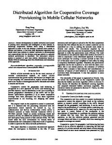
We run the consensus update (4) developed Section III for different numbers of agents m and the results are shown in Table I and the associated Fig. 2. Note that the larger the number of agents, the better the approximation of the sought expectation S ⋆ , as predicted by the law of large numbers. Furthermore, choosing the weights αij uniformly results in a better performance of the algorithm, as discussed in Section IV. Following is the final stochastic S for the case of m = 100 agents and uniform weights: .2501 .2813 .2502 0 0 0 0 0 0 .2183
.2432 .2674 .2638 .2257 0 0 0 0 0 0 0 .2079 .2484 .2916 .2521 0 0 0 0 0 0 0 .2377 .2514 .2867 .2242 0 0 0 0 0 0 0 .2313 .2311 .2797 .2580 0 0 0 0 0 0 0 .2302 .2473 .2871 .2354 0 0 0 0 0 0 0 .2487 .2415 .2654 .2443 0 0 0 0 0 0 0 .2134 .2422 .2746 .2698 .2619 0 0 0 0 0 0 .2570 .2313 .2498 .2448 .2434 0 0 0 0 0 0 .2498 .2620
Note that S approximates well the transition matrix S ⋆ with the the fastest mixing rate, which for the particular example has all positive entries equal to 0.25. VI. C ONCLUSIONS
TABLE I M ARKOV CHAIN SHOWN IN F IG . 1.
Random αi Uniform αi
Number of agents m 10 20 50 .8591 .7993 .7755 ±.0474 ±.0152 ±.0051 .8367 .7863 .7680 ±.0324 ±.0085 ±.0033
30
40
50
60
70
80
90
100
a novel distributed relaxation to the problem by constructing differential flows on the set of stochastic matrices. In particular, we defined a probability distribution over the set of stochastic matrices and associated an agent with any random matrix drawn from this distribution. Under the assumption that the network of agents is connected, we employed consensus to achieve agreement of all agents independent of their initial states. For sufficiently many agents, we showed that the asymptotic consensus limit converged to the mean stochastic matrix, which for the distribution under consideration, corresponded to the chain with the fastest mixing rate. The proposed distribution as well as the desired sparsity patterns, relied on results that express general stochastic matrices as convex combinations of 0-1 stochastic matrices. Due to its differential and distributed nature, our approach can handle large problems and seems likely to be well suited for applications in distributed control and robotics. Future work involves determining more quantitative bounds on the number of agents required to obtain almost optimal solutions, as well as applications in distributed robotics, in the context of probabilistic mapping of environments and target tracking.
T HE COST FUNCTION ψ(S) AFTER APPLYING CONSENSUS (4) FOR THE
5 .9678 ±.0636 .9252 ±.0472
20
Fig. 2. Plot of the cost function ψ(S) obtained by applying consensus (4) for the pattern illustrated in Fig. 1, corresponding to the data presented in Table I. Note that the larger the number of agents, the better the approximation of the sought expectation S ⋆ . Moreover, uniform weights αij ≥ 0 result in better performance, as discussed in Section IV. The communication networks G underlying the consensus algorithm are taken to be random and connected.
In this paper, we considered the problem of determining the fastest mixing Markov chain with a desired sparsity pattern, captured by a stochastic transition matrix. We developed
ki = 5, ∀ i
10
Number of agents m
uniformly, as discussed in Section IV. Following is the initial stochastic matrix Si of a sample agent i: .2 0 .4 0 0 0 0 0 0 .4 00 Si = 00 0
0
100 .7605 ±.0012 .7587 ±.0010
1440
R EFERENCES [1] L. Billera, and P. Diaconis. A Geometric Interpretation of the Metropolis-Hastings Algorithm, Statistical Science, vol. 16, pp. 335– 339, Nov. 2001. [2] W. Hastings. Monte Carlo Sampling Methods using Markov Chains and their Applications, Biometrika, vol. 57, pp. 97–109, 1970. [3] W. R. Gilks, S. Richardson, and D. Spiegelhalter. Markov Chain Monte Carlo in Practice: Interdisciplinary Statistics, Chapman and Hall, 1996. [4] G. Casella, and E. I. George. Explaining the Gibbs Sampler, The American Statistician, vol. 46(3), pp. 167–174, 1992. [5] S. Chib, and E. Greenberg. Markov Chain Monte Carlo Simulation Methods in Econometrics, Econometric Theory, vol. 12(3), pp. 409– 431, 1996.
[6] Z. Yang, and B. Rannala. Bayesian Phylogenetic Inference using DNA Sequences: A Markov Chain Monte Carlo Method, Molecular Biology and Evolution, vol. 14, pp. 717–724, 1997. [7] C. J. Geyer, and E. A. Thompson. Annealing Markov Chain Monte Carlo with Applications to Ancestral Inference, Journal of American Statistical Association, vol. 90(431), pp. 909–920, 1995. [8] S. Thrun, D. Fox, W. Burgard, and F. Dellaert. Robust Monte Carlo Localization for Mobile Robots, Artificial Intelligence, vol. 128(1-2), pp. 99-141, May 2001. [9] C. Hue, J.-P. Le Cadre, and P. Perez. Sequential Monte Carlo Methods for Multiple Target Tracking and Data Fusion, IEEE Transactions on Signal Processing, vol. 50(2), pp. 309–325, Feb. 2002. [10] M. Kaess, and F. Dellaert. A Markov Chain Monte Carlo Approach to Closing the Loop in SLAM, Proc. of the IEEE Conference on Robotics and Automation, Barcelona, Spain, April 2005, pp. 643–648. [11] D. Marinakis, G. Dudek, D. J. Fleet. Learning Sensor Network Topology through Monte Carlo Expectation Maximization, Proc. of the IEEE Conference on Robotics and Automation, Barcelona, Spain, April 2005, pp. 4581–4587. [12] A. Ranganathan, and F. Dellaert. Inference in the Space of Topological Maps: An MCMC-Based Approach, Proc. of the IEEE/RSJ International Conference on Intelligent Robots and Systems, Sendai, Japan, Sept. 2004, pp. 1518–1523. [13] C.-X. Shi, B.-R. Hong, and Y.-Q. Wang. Cooperative Exploration by Multi-Robots without Global Localization, International Journal of Advanced Robotic Systems, vol. 5(2), pp. 129–138, 2008. [14] J. Liu. Monte Carlo Strategies in Scientific Computing. Springer Series in Statistics. Springer-Verlag, New York, 2001. [15] P. Bremaud. Markov Chains, Gibbs Fields, Monte Carlo Simulation and Queues. Texts in Applied Mathematics. Springer-Verlag, BerlinHeidelberg, 1999. [16] C. J. Geyer. Practical Markov Chain Monte Carlo. Statistical Science, vol. 7(4), pp. 473–483, Nov. 1992. [17] S. Chib, and E. Greenberg. Understanding the Metropolis-Hastings Algorithm, The American Statistician, vol. 49(4), pp. 327–335, Nov. 1995. [18] S. Boyd, P. Diaconis, and L. Xiao. Fastest Mixing Markov Chain on a Graph. SIAM Review, vol. 46(4), pp. 667–689, Dec. 2004. [19] D. Aldous. Random Walk on Finite Groups and Rapidly Mixing Markov Chains. In Seminaire de Probabilities XVII, volume 986 of Lecture Notes in Mathematics, pp. 243–297. Springer, New York, 1983. [20] P. Diaconis. Group Representations in Probability and Statistics. IMS, Hayward, CA, 1988. [21] M. Jerrum, and A. Sinclair. Approximating the Permanent. SIAM Journal on Computing, vol. 18, pp. 1149–1178, 1989. [22] P. Diaconis, and D. Stroock. Geometric Bounds for Eigenvalues of Markov Chains. The Annals of Applied Probability, vol. 1(1), pp. 36– 61, 1991. [23] A. Sinclair. Improved Bounds for Mixing Rates of Markov Chains and Multicommodity Flow. Combinatorics, Probability and Computing, vol. 1, pp. 351–370, 1992.
[24] N. Kahale. A Semidefinite Bound for Mixing Rates of Markov Chains. Proc. of the 5th Integer Programming and Combinatorial Optimization Conference, Springer Lecture Notes in Computer Science, vol. 1084, pp. 190–203, 1996. [25] G. Grimmett, and D. Stirzaker. Probability and Random Processes. Oxford University Press, New York, 2003 (third edition). [26] W. Feller. An Introduction to Probability Theory and its Applications, Vol. 1. John Wiley & Sons, 1968 (third edition). [27] A. Berman, and R. J. Plemmons. Nonnegative Matrices in the Mathematical Sciences. SIAM Classics in Applied Mathematics, Philadelphia, 1994. [28] C. Godsil, and G. Royle. Algebraic Graph Theory, Springer-Verlag, New York, 2001. [29] R. G. Laha, and V. K. Rohatgi. Probability Theory, pp. 446-451, John Wiley and Sons, 1979.
A PPENDIX In this section we show a generalization of the well known identity Var(aX + bY ) = a2 Var(X) + b2 Var(Y ) [25] for X, Y ∈ R independent identically distributed random variables, to the case of random vectors. In particular, we have the following result. Lemma 1.1: Let X, Y ∈ Rn be independent identically distributed random vectors with mean E(X) = E(Y ) = µ ∈ Rn and let Var(X) , EkX − E(X)k22 (similarly for Y ) [29, pp. 446–451]. Then, Var(aX + bY ) = a2 Var(X) + b2 Var(Y ), for any scalars a, b ∈ R. Proof: Observe first that Var(X) = E(X − µ)T (X − µ)
= E(X T X) − 2E(X T )µ + µT µ = EkXk22 − kµk22 ,
and similarly Var(Y ) = EkY k22 − kµk22 . Then,
Var(aX + bY ) = EkaX + bY − E(aX + bY )k22 = EkaX + bY − (a + b)µk22
= EkaX + bY k22 − (a + b)2 kµk22
= a2 EkXk22 + 2abE(X T )E(Y ) + b2 EkY k22 − (a + b)2 µ2 � � = a2 EkXk22 − kµk22 + b2 EkY k22 − kµk22 = a2 Var(X) + b2 Var(Y ),
which completes the proof.
1441