A distributed load balancing algorithm for climate big data processing ...
Recommend Documents
During gateway uptime. All gateways apply GWLB when: .... generated at a Internet server and sent to a varying number of randomly chosen sinks in the WMN, ...
high, and due to limited wireless link capacity, gateways are likely to become a ... and can improve network utilization in both balanced and skewed topologies.
Keywords Virtual machine; task scheduling; workload; makespan time; load balancing ; ..... [14] A. Thomas et. al., "Credit Based Scheduling Algorithm in Cloud ...
the cost sustained to reach its destination by a proper flow assignment. Practically speaking, a single packet of the flow could be approximately considered as an ...
Apr 3, 2015 - [email protected], [email protected]. AbstractâWe study the problem of load balancing in dis- tributed stream processing engines, ...
Mar 9, 2015 - represented by mobile agents, are associated in a parallel virtual layer, ... load balancing procedure is performed by the virtual host agent.
takes up to several minutes. In contrast to this the startup ... Docker Swarm) are monolithic applications running as daemons on dedicated nodes of the cloud.
The remaining parts of this paper are organised as ... represented in slot format with (start-time, finish-time). .... algorithm is O(nlogm) using priority queue data.
Journal of Geographic Information System, 2011, 3, 128-139 ... load balancing for D-GIS in order to quickly render information to client interface by involving a ...
Proxy. 2. NCC W 21G 1GB P-III. FreeBSD. 4.11. Proxy. 3. IBM. Netfinity. 5500. S 12G 512MB. P-III. 450 Ã. 2. FreeBSD. 3.4. Proxy. 01. Domain W 12G 512MB P-III.
KEYWORDS. Job Processing, Load Balancing, Monitoring, Distributed And Scalable. 1. ..... Thus, on a high end server, the same processor can be configured to ...
Keywords: Distributed Control, Load Balancing, Software Agents, Multiagent ... Demand Side Management (DSM), i.e., actions taken on the customer's side to ...
ABSINTHE (Agent-based monitoring and control of district heating systems) [6] is a collaboration project between Blekinge Institute of Technology and ...
the current node and its neighboring nodes. For calculating the current load on a node, the following parameters are considered. â¢. CPU Idle time (NIt).
algorithm is a Hybrid algorithm (HACOBEE) which is the optimal solution for load ... Keywords: Ant Colony Optimization, Artificial Bee Colony, Cloud Computing, ...
load on fogs a new load balancing technique Shortest Load First(SLF) is .... also faces some latency issues due to the huge geographical distance of clouds.
Next generation of algorithm trading will be big data driven. This paper presents the big data processing platform for algorithm trading strategy evaluation, which ...
type of application, there are important performance concerns that need to be ... performance issues relating to these types of networks are discussed. .... The SCF Proxy accepts INAP IDL invocations from the UAP and GSEP, transfers ... (protocol enc
[7l Ahmed K. Ezzat, R. Daniel Bergenon and John L Po- koski, âTask Allocation ... [12] E J. MacWilliams and N. J. A. Sloane, The Theory of. Emr-Comting Codes ...
scalability, availability and reliability of web servers to .... In this approach, the domain name system ... of servers that must be in a domain, in essence the policy.
Dec 20, 1996 - Reinforcement Learning for ... learning and a linear value-function approximator. In .... During each quantum, once the work has been al-.
distributed computing. In general, the goal of load balancing is to dynamically distribute some set of tasks or jobs among a number of processing nodes in such a.
AContent Delivery Network (CDN) represents a popular and useful solution to effectively support emerging Web applications by adopting a distributed overlay of ...
Nov 15, 2009 - Suppose that customers arrive to a service center (call center, web server, etc.) ... show that these results lead to heuristics that perform well.
A distributed load balancing algorithm for climate big data processing ...
Mar 24, 2016 - The load imbalance has a serious impact on the processing speed of ... big data; data processing; load imbalance; optimization algorithm; high ...
CONCURRENCY AND COMPUTATION: PRACTICE AND EXPERIENCE Concurrency Computat.: Pract. Exper. 2016; 28:4144–4160 Published online 24 March 2016 in Wiley Online Library (wileyonlinelibrary.com). DOI: 10.1002/cpe.3822
SPECIAL ISSUE PAPER
A distributed load balancing algorithm for climate big data processing over a multi-core CPU cluster Yuzhu Wang1,2,*,†, Jinrong Jiang2, Huang Ye2 and Juanxiong He3 1
Institute of Remote Sensing and Digital Earth, Chinese Academy of Sciences, Beijing, China 2 Computer Network Information Center, Chinese Academy of Sciences, Beijing, China 3 Institute of Atmospheric Physics, Chinese Academy of Sciences, Beijing, China
big data; data processing; load imbalance; optimization algorithm; high performance computing
1. INTRODUCTION The Earth System Model (ESM) is a coupled climate model which is employed to simulate the Earth’s climate states in different periods. Many countries have developed their own ESMs. One of the most famous ESMs is the Community Earth System Model (CESM) which is mainly developed by the National Center for Atmospheric Research (NCAR) of the United States [1]. In China, there are five ESMs which have been used for the Fifth Assessment Report of the United Nations Intergovermental Panel on Climate Change (IPCC AR5) [2]. It indicates that China has good competencies in developing ESMs at present. The Chinese Academy of Sciences-Earth System Model (CAS-ESM) has been developed by the Institute of Atmospheric Physics (IAP) of Chinese Academy of Sciences (CAS) [3, 4]. And the CAS-ESM system has achieved the nesting (or coupling) of the Institute of Atmospheric Physics of Chinese Academy of Sciences Atmospheric
2. MODELING SYSTEM The CAS-ESM is designed and developed based on the CESM version 1.0. The CAS-ESM is composed of six separate component models and one central coupler component. It can be employed to conduct fundamental research for the Earth’s climate states. In the CAS-ESM system, the atmosphere component model used is the IAP AGCM4.0 which is developed by the IAP, the ocean component model is the LASG/IAP Climate System Ocean Model (LICOM) version 2.0 developed by the State Key Laboratory of Numerical Modeling for Atmospheric Sciences and Geophysical Fluid Dynamics (LASG) of the IAP, the land component model is the Common Land Model (CoLM) which is developed by Beijing Normal University, the sea-ice component model is the CICE version 4, the land-ice component model is the GLC and the atmospheric chemical component model is the Global Environmental Atmospheric Transport Model (GEATM) developed by the IAP. Besides the six separate model components, the Advanced Research WRF version 3.2 is put into the CAS-ESM modeling system. Here, the WRF is considered as a part of the IAP AGCM4.0 source code. Meanwhile, the four computation modules (GEOGRID, METGRID, REAL, INTEGRATION) of the WRF are integrated together in order to make the IAP AGCM4.0 drive the WRF online. That means that the IAP AGCM4.0 provides the initial conditions, lateral boundary conditions, surface temperature and soil moisture online to the WRF. The data exchange between the IAP AGCM4.0 and WRF is achieved through the CAS-ESM Coupler version 7 (CPL7). The model structure of the CAS-ESM system is presented in Figure 1. Figure 2 illustrates the flow chart of time integration of the WRF in the CAS-ESM. The coupling time interval between the IAP AGCM4.0 and CPL7 is atm_cpl_dt, and the one between the WRF and CPL7 is wrf_cpl_dt. The wrf_cpl_dt can be set to the IAP AGCM4.0 time step or an integral multiple of the IAP AGCM4.0 and WRF time steps. When the CPL7 sends the data to the WRF at each time step of data exchange, the lateral boundary data set and other data information of the WRF are updated [25].
3. PROBLEM DESCRIPTION AND ANALYSIS 3.1. METGRID module The METGRID program or computation module is mainly used to interpolate meteorological data with intermediate-format onto the computation grid. The GEOGRID (geoscientific grid) program defines simulation domains. The METGRID.TBL file controls interpolation methods of every meteorological field. Average_4pt, wt_average_4pt, search_extrap and the other interpolation
Figure 2. Flow chart of time integration of the WRF in the CAS-ESM.
methods are often utilized. Among these interpolation methods, the search_extrap method represents breadth-first search interpolation. Normally, a computation grid in climate models is a grid cell that denotes a physical region of the earth. When a parent grid cell with low resolution is divided into several son grid (or subgrid) cells with high resolution, land or sea information on son grid cells may be missing or masked. For example, a vertex on a low-resolution parent grid represents a data point with land information, while the same vertex on a high-resolution son grid might represent a data point with sea information. Therefore, the vertex can get the sea data information by using some interpolation methods. In the METGRID module, the breadth-first search interpolation method is used to find the nearest valid (not missing or masked) vertex of the invalid point (x, y). Then the value of the valid vertex is assigned to the point (x, y) [29].
Figure 3. The METGRID running time of all the 64 MPI ranks.
Through the testing, it is found that the load imbalance of the METGRID is related to the function search_extrap which is called by the METGRID for many times. In the five days numerical simulation, the subroutine METGRID module is called for 2161 times circularly. Figure 4 shows all the time spent on executing the search_extrap during calling the METGRID for 2161 times. According to Figure 4, the search_extrap running time of each process which accounts for a significant portion of the METGRID running time is also quite unbalanced and the changing trend of the search_extrap running time from MPI rank 0 to 63 is consistent with the METGRID running time. Therefore, the conclusion is that the load imbalance of the search_extrap running time for each process results in the load imbalance of the METGRID directly. 3.3. Function search_extrap The function search_extrap is used to find the nearest valid neighbor of an invalid vertex which represents a missing or masked source data point. Table I illustrates the pseudocode of the search_extrap. To find out the reason of the load imbalance in the search_extrap further, the total number of times that the search_extrap is invoked by the METGRID is counted. As shown in Table I, the function
Table I. Function search_extrap. Algorithm 1 Search_extrap before the optimizing Input: xx,yy,izz: Coordinate of interpolating point array: Three dimensional array representing the input field start_x,end_x: Start-end value of x-coordinate in the domain mesh start_y,end_y: Start-end value of y-coordinate in the domain mesh start_z,end_z: Start-end value of z-coordinate in the domain mesh msgval: A real number giving the value in the input field that is assumed to represent missing data maskval: A real number giving the value in the interpolation mask that is assumed to represent missing data mask_array: Two dimensional array representing the interpolation mask Output: search_extrap: Field data at the point nearest to (xx, yy) that has a non-missing value 1: found_valid = false 2: qdata%x = nint(xx), qdata%y = nint(yy), call q_insert(q, qdata) 3: for q is not empty and found_valid is false do 4: assign the first element of the queue q to the variable qdata, then remove the first element of q 5: i = qdata%x, j = qdata%y 6: if present(mask_array) and present(maskval) do 7: if (array(i, j, izz) /= msgval and mask_array(i, j) /= maskval) found_valid = true 8: else do 9: if (array(i, j, izz) /= msgval) found_valid = true 10: end if 11: if (i-1 > = start_x or i + 1 < = end_x or j-1 > = start_y or j + 1 < = end_y) do 12: qdata%x = i-1 or i + 1 or i or i, qdata%y = j or j or j-1 or j + 1, call q_insert(q, qdata) 13: end if 14: end for 15: if found_valid is true do 16: continue do the second for-loop to find the nearest point (x, y) to (xx, yy) from the queue q that has a nonmissing value 17: search_extrap = array(x, y) 18: else do 19: search_extrap = msgval 20: end if 21: return search_extrap
search_extrap includes two for-loops. Therefore, the total numbers of the first for-loop and the second for-loop are also counted to find which for-loop leads to the load imbalance of the search_extrap. The total number of times that the search_extrap is invoked by the METGRID is different for each process as illustrated in Figure 5, but the direct relevance between it and the load imbalance is not obtained. Figure 6 indicates that from MPI rank 0 to 63 there is a really big disparity in the total number of loops inside the search_extrap and the changing trend of all the amount of loops is consistent with the METGRID running time in Figure 3. So Figure 6 supports the conclusion in Section 3.2 further. Meanwhile, Figure 6 shows that the total amount of the first loop accounts for a main part of all the amount of loops. Therefore, it is the best method for solving the load imbalance problem to decrease the total amount of the first loop in the search_extrap.
Figure 5. The total number of times that the search_extrap is called by each MPI rank.
the search_extrap is called by the METGRID each time, because frequent iterations will take too much time. To reduce the number of iterations, the idea of the optimizing algorithm is that each process stores the traversal record of executing the first for-loop code for all the vertexes before the search_extrap is called for the first time. When the search_extrap is called later, each process reads the traversal record instead of executing the first loop again. In this way, the total amount of the first loop in the search_extrap can be decreased effectively. In theory, the problem of the load imbalance should be solved effectively. 4.2. Algorithm implementation Although the values of the mask_array for each process are the same, the maskval may be different. But the value of the maskval is either 0 or 1. Therefore, each process has two traversal records. Based on the algorithm idea above, a new subroutine named search_match_mask and six common variables that are the arrays match_mask_array0, match_mask_array1, match_mask_queue0, match_mask_queue1, match_mask_found_valid0 and match_mask_found_valid1 need to be created. The subroutine search_match_mask is used to find the nearest valid neighbor of every vertex in the grid and then
store the traversal record. The variable match_mask_array0 is used to store the coordinate of the nearest valid neighbor of every vertex when the value of the maskval is 0. In the same way, the variable match_mask_array1 is used to store the coordinate of the nearest valid neighbor of every vertex when the value of the maskval is 1. The variable match_mask_queue0 is used to store the queue q during searching the nearest valid neighbor of every vertex when the value of the maskval is 0. The variable match_mask_queue1 is used to store the queue q during searching the nearest valid neighbor of every vertex when the value of the maskval is 1. The queue q can be used for the computing in the second for-loop in the function search_extrap. The variable match_mask_found_valid0 is used to record whether to find the valid neighbor of a vertex when the value of the maskval is 0. The variable match_mask_found_valid1 is used to record whether to find the valid neighbor of a vertex when the value of the maskval is 1. The detailed optimizing algorithm implementation is shown in Table II. Before the search_extrap is called by each process for the first time, each process calls the subroutine search_match_mask at first, and then assigns the traversal records to the two dimensional arrays match_mask_array0, match_mask_array1, match_mask_queue0, match_mask_queue1, match_mask_found_valid0 and match_mask_found_valid1. In addition, the corresponding code in the function search_extrap is modified, as shown in Table III. After the optimizing above, the total amount of loops in the search_extrap is reduced greatly. And the total running time of the search_extrap should be decreased drastically, too.
Table II. Subroutine search_match_mask. Algorithm 2 Search_match_mask Input: match_mask_array_tmp0: Two dimensional array storing the coordinates of the nearest valid neighbor match_mask_array_tmp1: Two dimensional array storing the coordinates of the nearest valid neighbor match_mask_queue_tmp0: Two dimensional array storing the corresponding valid queue match_mask_queue_tmp1: Two dimensional array storing the corresponding valid queue match_mask_found_valid_tmp0: Two dimensional logical array match_mask_found_valid_tmp1: Two dimensional logical array start_x,end_x: Start-end value of x-coordinate in the domain mesh start_y,end_y: Start-end value of y-coordinate in the domain mesh mask_array: Two dimensional array representing the interpolation mask Output: match_mask_array_tmp0, match_mask_array_tmp1, match_mask_queue_tmp0, match_mask_queue_tmp1, match_mask_found_valid_tmp0, match_mask_found_valid_tmp1 1: for k = 0, 1 do 2: for im = start_x, start_x + 1, start_x + 2, …, end_x do 3: for jm = start_y, start_y + 1, start_y + 2, …, end_y do 4: if (k == 0) do 5: found_valid = false 6: qdata%x = im, qdata%y = jm, call q_insert(match_mask_queue_tmp0(im, jm), qdata) 7: for match_mask_queue_tmp0(im, jm) is not empty and found_valid is false do 8: assign the first element of the queue match_mask_queue_tmp0(im, jm) to the variable qdata, then remove the first element of the queue 9: i = qdata%x, j = qdata%y 10: if (mask_array(i, j) /= k) do 11: found_valid = true 12: match_mask_array_tmp0(im, jm)%x = i 13: match_mask_array_tmp0(im, jm)%y = j 14: end if 15: if (i-1 > = start_x or i + 1 < = end_x or j-1 > = start_y or j + 1 < = end_y) do 16: qdata%x = i-1 or i + 1 or i or i, qdata%y = j or j or j-1 or j + 1 17: call q_insert(match_mask_queue_tmp0(im, jm), qdata) 18: end if 19: end for 20: match_mask_found_valid_tmp0(im, jm) = found_valid 21: else if (k == 1) do 22: change match_mask_queue_tmp0 into match_mask_queue_tmp1, change match_mask_array_tmp0 into match_mask_array_tmp1, and change match_mask_found_valid_tmp0 into match_mask_found_valid_tmp1, then do the same operation with k == 0 23: end if 24: end for 25: end for 26: end for
Table III. Function search_extrap after the optimizing. Algorithm 3 Search_extrap after the optimizing Input: xx,yy,izz: Coordinate of interpolating point array: Three dimensional array representing the input field start_x,end_x: Start-end value of x-coordinate in the domain mesh start_y,end_y: Start-end value of y-coordinate in the domain mesh start_z,end_z: Start-end value of z-coordinate in the domain mesh msgval: A real number giving the value in the input field that is assumed to represent missing data maskval: A real number giving the value in the interpolation mask that is assumed to represent missing data mask_array: Two dimensional array representing the interpolation mask Output: search_extrap: Field data at the point nearest to (xx, yy) that has a non-missing value 1: found_valid = false 2: im = nint(xx), jm = nint(yy) 3: if present(mask_array) and present(maskval) do 4: if (maskval == 0) do 5: if match_mask_found_valid0(im, jm) is true do 6: i = match_mask_array0(im, jm)%x 7: j = match_mask_array0(im, jm)%y 8: if (array(i, j, izz) /= msgval) do 9: found_valid = true 10: call q_copy(match_mask_queue0, q_temp) 11: execute the second loop in the original function search_extrap and change q into q_temp 12: stop the function search_extrap 13: else do 14: execute the code of the original function search_extrap 15: end if 16: else do 17: search_extrap = msgval 18: stop the function search_extrap 19: end if 20: else if (maskval == 1) do 21: change match_mask_queue0 into match_mask_queue1, change match_mask_array0 into match_mask_array1, and change match_mask_found_valid0 into match_mask_found_valid1, then do the same operation with maskval == 0 22: end if 23: end if 24: return search_extrap
Because there is a MPI_Barrier operation before the WRF integration, the total running time of the METGRID and REAL modules for each MPI rank is the same. Table IV compares not only the total running time of the CAS-ESM but also the one of the METGRID and REAL modules before and after the optimizing. Here, the WRF uses the default decomposition strategy. From Table IV, the study draws some conclusions as follows. 1. The running time of the METGRID and REAL modules before the optimizing takes up over 70% of the total running time of the CAS-ESM. Therefore, it explains further the importance of making the optimization for the METGRID. 2. When running the CAS-ESM on 64 CPU cores, the total computing speed of the METGRID and REAL modules after the optimizing is about 7.2 times faster than before. Moreover, the total computing speed of the CAS-ESM after the optimizing improves by 217.53%. 3. When the CAS-ESM is run again on different numbers of CPU cores, the METGRID and REAL modules after the optimizing can achieve a similar speedup. 4. The performance improvement peaks on 64 cores. When the number of the cores used is constant, all the amount of loops of MPI rank 0 in the search_extrap is the most in all the MPI ranks as shown in Figure 6, so MPI rank 0 can have a major impact on the running time of the METGRID and REAL modules. The number of times that the search_extrap is invoked by the METGRID, all the amount of loops and the amount of the first for-loop in the search_extrap for MPI rank 0 before the optimizing are shown in Table V. From 16 cores to 256 cores, the current number of times that the search_extrap is called by MPI rank 0 is almost half of the former, but the amount of the first for-loop from 32 cores to 64 cores only decreases slightly. This is because MPI rank 0 on 64 cores needs more loops to finish the breadth-first search interpolation for its invalid grid vertexes. When the number of the cores used is different, the grid domain that is processed by each MPI rank 0 is also different. The amount of the first for-loop of MPI rank 0 is related to its own grid domain (or subdomain) processed. Similarly, the running time of the METGRID and REAL modules from 32 cores to 64 cores only decreases a little. That means that the load imbalance of the METGRID on 64 cores is worse. In this situation, the optimizing
Table V. The details about the number of the loops inside the function search_extrap for MPI rank 0 before the optimizing. The all_search_number is the total number of times that the search_extrap is called by MPI rank 0; the all_loops_number is all the amount of loops for MPI rank 0 and the all_loop1_number is the total amount of the first for-loop for MPI rank 0. Nodes (cores)
Figure 8. The precipitation (mm) at 00 UTC 5 March. (a) Before the optimizing, (b) after the optimizing. The black dot is the center of the SGP site.
algorithm can make better use of its advantage. Therefore, the performance improvement can peak on 64 cores. In the algorithm proposed above, six common arrays (match_mask_array0, match_mask_array1, match_mask_queue0, match_mask_queue1, match_mask_found_valid0 and match_mask_found_valid1) need to be created. Whichever case the CAS-ESM system simulates, the size of each array is 128 × 261. Therefore, the six arrays need about 3 MB memory space. Today, each node of a cluster usually shares greater than or equal to 64 GB memory, so generally the size of memory capacity will not affect the performance of the optimizing algorithm. The ratio of the running time of the METGRID and REAL modules before and after the optimizing can be written as
Figure 9. Speedup of the METGRID and REAL modules.
Figure 10. Parallel efficiency of the METGRID and REAL modules.
number. Comparing with the 16 CPU cores, after the optimizing the speedup of METGRID and REAL modules with 45.99% parallel efficiency on 256 CPU cores can reach 7.36, as shown in Figures 9 and 10. Obviously, the optimizing algorithm improves the speedup and parallel efficiency of the METGRID and REAL modules. On the whole, the METGRID and REAL modules in the CASESM have desirable parallel performance and strong scalability.
before. The considerable improvement of the computing speed for the METGRID and REAL modules is quite meaningful for the real-time climate simulation of the CAS-ESM. Besides, the nesting process of the IAP AGCM4.0 and WRF by the CPL7 in the CAS-ESM is described. Based the parallel analysis, the METGRID and REAL modules in the CAS-ESM have desirable parallel performance and strong scalability. In the future, the system with thousands of CPU cores on larger clusters will be evaluated. And the METGRID module and the CAS-ESM system could still continue to be optimized in order to achieve to higher parallel performance. Although there are few application researches on big data of climate models or earth system models, we can try them later by using programming models of big data with the coming of big data era. Graphics processing units (GPUs) are often used for large-scale or data-intensive computing applications [31–35], so it will be also considered to develop the GPU version of the algorithm later in order to improve the data processing ability of the METGRID module further. ACKNOWLEDGEMENTS
20. Xu Z, Wei X, Luo X, Liu Y, Mei L, Hu C, Chen L. Knowle: a semantic link network based system for organizing large scale online news events. Future Generation Computer Systems 2015; 43:40–50. 21. Johnsen P, Straka M, Shapiro M, Norton A, Galarneau T. Petascale WRF simulation of hurricane sandy: deployment of NCSA’s cray XE6 blue waters. Proceedings of the International Conference on High Performance Computing, Networking, Storage and Analysis (SC), 2013. 22. Ding Z, Guo D, Liu X, Luo X, Chen G. A MapReduce-supported network structure for data centers. Concurrency and Computation: Practice and Experience 2012; 24(12):1271–1295. 23. Wang L, Tao J, Ranjan R, Marten H, Streit A, Chen J, Chen D. G-Hadoop: MapReduce across distributed data centers for data-intensive computing. Future Generation Computer Systems 2013; 29(3):739–750. 24. Zhang H, Zhang M, Zeng Q. Sensitivity of simulated climate to two atmospheric models: Interpretation of differences between dry models and moist models. Monthly Weather Review 2013; 141(5):1558–1576. 25. He J, Zhang M, Lin W, Colle B, Liu P, Vogelmann AM. The WRF nested within the CESM: simulations of a midlatitude cyclone over the Southern Great Plains. Journal of Advances in Modeling Earth Systems 2013; 5(3):611–622. 26. Michalakes J, Dudhia J, Gill D, et al. The weather research and forecast model: software architecture and performance. Proceedings of the 11th ECMWF Workshop on the Use of High Performance Computing In Meteorology, 2004; 156–158. 27. Shainer G, Liu T, Michalakes J, Liberman J, et al. Weather Research and Forecast (WRF) model performance and profiling analysis on advanced multi-core HPC clusters. The 10th LCI International Conference on HighPerformance clustered Computing, Boulder, CO, 2009. 28. Malakar P, Saxena V, George T, et al. Performance evaluation and optimization of nested high resolution weather simulations. In Euro-Par 2012 Parallel Processing. Springer: Berlin Heidelberg, 2012; 805–817. 29. Wang W, Bruyère C, Duda M, et al. ARW version 3 modeling system user’s guide. Mesoscale & Miscroscale Meteorology Division, National Center for Atmospheric Research, 2010. 30. Xie S, Zhang M, Branson M, et al. Simulations of midlatitude frontal clouds by single-column and cloud-resolving models during the atmospheric radiation measurement March 2000 cloud intensive operational period. Journal of Geophysical Research 2005; 110, D15S03. DOI: 10.1029/2004JD005119.. 31. Chen D, Li X, Wang L, Khan SU, Wang J, Zeng K, Cai C. Fast and scalable multi-way analysis of massive neural data. IEEE Transactions on Computers 2015; 64(3):707–719. 32. Chen D, Li D, Xiong M, Bao H, Li X. GPGPU-aided ensemble empirical-mode decomposition for EEG analysis during anesthesia. IEEE Transactions on Information Technology in Biomedicine 2010; 14(6):1417–1427. 33. Chen D, Wang L, Ouyang G, Li X. Massively parallel neural signal processing on a many-core platform. Computing in Science & Engineering 2011; 13(6):42–51. 34. Chen D, Wang L, Zomaya AY, Dou M, Chen J, Deng Z, Hariri S. Parallel simulation of complex evacuation scenarios with adaptive agent models. IEEE Transactions on Parallel and Distributed Systems 2015; 26(3):847–857. 35. Yang C, Xue W, Fu H, Gan L, Li L, Xu Y, Lu Y, Sun J, Yang G, Zheng W. A peta-scalable CPU-GPU algorithm for global atmospheric simulations. Proceedings of the 18th ACM SIGPLAN Symposium on Principles and Practice of Parallel Programming, 2013; 1–12.