Multiuser Decoding for Coded CDMA. Bin Hu, Ingmar Land, Lars Rasmussen, Romain Piton, and Bernard H. Fleury. AbstractâIn this paper, a theoretical ...
432
IEEE JOURNAL ON SELECTED AREAS IN COMMUNICATIONS, VOL. 26, NO. 3, APRIL 2008
A Divergence Minimization Approach to Joint Multiuser Decoding for Coded CDMA Bin Hu, Ingmar Land, Lars Rasmussen, Romain Piton, and Bernard H. Fleury
Abstract—In this paper, a theoretical framework of divergence minimization (DM) is applied to derive iterative receiver algorithms for coded CDMA systems. The DM receiver obtained performs joint channel estimation, multiuser decoding, and noisecovariance estimation. While its structure is similar to that of many ad-hoc receivers in the literature, the DM receiver is the result of applying a formal framework for optimization without further simplifications, namely the DM approach with a factorizable auxiliary model distribution. The well-known expectationmaximization (EM) algorithm and space-alternating generalized expectation-maximization (SAGE) algorithm are special cases of degenerate model distributions within the DM framework. Furthermore, many ad-hoc receiver structures from literature are shown to represent approximations of the proposed DM receiver. The DM receiver has four interesting properties that all result directly from applying the formal framework: (i) The covariances of all estimates involved are taken into account. (ii) The residual interference after interference cancellation is handled by the noise-covariance estimation as opposed to by LMMSE filters in other receivers. (iii) Posterior probabilities of the code symbols are employed rather than extrinsic probabilities. (iv) The iterative receiver is guaranteed to converge in divergence. The theoretical insights are illustrated by simulation results. Index Terms—Variational Bayesian inference, divergence minimization, iterative receivers, multiuser decoding, channel estimation, interference cancellation, noise-covariance estimation, residual interference.
I. I NTRODUCTION
M
AXIMUM likelihood (ML) decoding of coded CDMA was first suggested in [1], where it was shown that the computational complexity grows exponentially with the product of the number of active users and the effective code constraint length. To reduce complexity, the dominant suboptimal approach so far has been to separate the multiuser detection and the decoding components, while allowing iterative exchange of information between the two [2]. Manuscript received June 1, 2007; revised October 28, 2007. The material has been presented in parts at IEEE Globecom ’07, Washington D.C., Dec 2630. This work has been supported in parts by RTX Telecom A/S, Denmark, the European Union Network of Excellence in Wireless Communications (NEWCOM), and the Australian Research Council under ARC Discovery Grant DP0663567 and ARC Communications Research Network (ACoRN) Grant RN0459498. B. Hu, I. Land, R. Piton, and B. H. Fleury are affiliated with the Department of Electronic Systems, Aalborg University, Denmark (e-mail: {bhu,il,rpi,bfl}@es.aau.dk). I. Land and L. K. Rasmussen are affiliated with the Institute for Telecommunications Research, University of South Australia, Australia (e-mail: {Ingmar.Land,Lars.Rasmussen}@unisa.edu.au). R. Piton is also affiliated with Motorola A/S, Mobile Devices Aalborg, Denmark. B. H. Fleury is also affiliated with Forschungszentrum Telekommunikation Wien (FTW), Austria. Digital Object Identifier 10.1109/JSAC.2008.080403.
Concatenated codes and iterative decoding inspired the canonical iterative joint multiuser decoder [3], [4], iterating between a multiuser a posteriori probability (APP) detector which ignores coding constraints, and individual channel code APP decoders, ignoring residual multiuser interference. The canonical decoder has subsequently been recognized as the application of the belief propagation (BP) algorithm to the factor graph corresponding to the posterior joint distribution for coded CDMA [5]. The factor graph inherently separates the multiuser APP detection problem and the individual APP decoder problems, providing justification for the canonical decoder structure. The marginalization of the joint distribution is then approximated through BP (message-passing), in terms of extrinsic probabilities, between the detection and the decoding components. The multiuser APP detector is also prohibitively complex, and thus an abundance of sub-optimal detectors have been considered for iterative multiuser decoding. Only a few formal optimization-based design frameworks are available for systematic design of sub-optimal detectors within an iterative multiuser decoder. Instead, receiver structures based on intuitive arguments have been proposed. Linear interference cancellation structures were shown to be particularly well suited for iterative joint multiuser decoding in [6]. Linear minimum mean-squared-error (LMMSE) filtering was subsequently proposed in [7], [8], [9], providing better performance at the expense of increased complexity. The resulting structure is linear cancellation followed by instantaneous LMMSE filtering. This approach has been further justified based on probabilistic data association (PDA) arguments in [10]. Formal design frameworks based on variational free energy have been proposed for the design of multiuser detectors specifically for iterative multiuser decoding. The variational free energy is similar to the Kullback-Leibler (KL) divergence (also called information divergence or cross entropy), measuring the similarity between a postulated auxiliary distribution and the desired posterior joint multiuser distribution. The postulated distribution minimizing the KL divergence also minimizes the variational free energy. Yedidia et. al. showed that, when the Bethe approximation is considered for the variational free energy [11], the zerogradient points of the Bethe free energy are the stationary points of the BP algorithm [12], [13], applied to the corresponding factor graph. The Bethe free energy, however, is not a convex function and thus, the zero-gradient points are not guaranteed to minimize the free energy. In addition, the messages from the multiuser APP detector requires the computation of the posterior joint distribution for the uncoded case,
c 2008 IEEE 0733-8716/08/$25.00 �
HU et al.: A DIVERGENCE MINIMIZATION APPROACH TO JOINT MULTIUSER DECODING FOR CODED CDMA
which is intractable [5], [14], [15]. Further simplifications to the message computation are introduced in [14], [15], leading to messages being determined by a chip-based cancellation structure similar to the schemes in [10]. A different framework is obtained based on variational Bayesian inference as proposed by Attias in [16]. Beal subsequently introduced the concept of complete data (known from the expectation-maximization (EM) algorithm [17]) into the variational Bayesian framework to formulate the variational Bayesian EM (VBEM) algorithm [18]. The minimization of the variational free energy becomes particularly tractable under the mean-field approximation, where the postulated auxiliary distribution is restricted to functions that can be factorized. For single-user MIMO systems, Christensen et al. propose an iterative receiver based on the VBEM algorithm for data and parameter estimation [19]. In [20] the BP algorithm is applied for message-passing in coded CDMA, where multiuser detection is based on the variational inference framework. Following this approach, the structures in [6] and [7] are formally justified as solutions to variational energy minimization, equivalent to divergence minimization, based on particular postulated auxiliary distribution functions. Conveniently the EM algorithm and the space-alternating generalized EM (SAGE) algorithm [21], representing a formal optimization framework in their own right, are special cases of the VEM/VBEM algorithms. In summary, there are three families of iterative multiuser decoder receivers originating from a pre-conceived iterative receiver structure based on intuitive design principles, minimization of the Bethe free energy, and minimization of the variational free energy, respectively. The same classification can be imposed on the iterative receiver structures proposed for joint multiuser channel estimation and decoding. A significant subset of joint multiuser channel estimation and decoding receivers suggested in the literature is based on a pre-conceived structure with a channel estimator, a multiuser interference cancellation detector, and a bank of single-user APP channel decoders [22], [23], [24], [25], [26]. A structure based on these three components makes intuitive sense, but lacks a formal justification. Some level of rigorous justification has been obtained by applying the EM and SAGE frameworks for the design of receivers [27], [28], [29]. However, these algorithms are based on hard decisions, and within the rigorous EM/SAGE framework the formal use of soft symbols in place of the hard decisions is not possible. The soft-symbol versions of EM and SAGE are therefore based on modifications, violating the original framework in order to accommodate the use of soft symbols [30], [31], [32]. As a consequence, none of the formal design frameworks are able to incorporate APP decoding as part of the rigorous optimization process. Motivated by the lack of a formal optimization framework for handling soft-symbol processing, and inspired by the development of the VBEM algorithm, we propose a closely related design framework based on KL divergence minimization (DM). Our main contribution is to develop and apply a systematic, holistic framework for designing joint multiuser channel estimation and decoding receivers. To our knowledge, no formal optimization framework has yet been suggested
433
for this task, capable of taking channel code constraints into account, as well as allowing for soft-symbol processing. The developed framework is based entirely on divergence minimization, updating an auxiliary model of the desired posterior distribution, and does not make any prior assumptions regarding receiver structure or signal processing techniques. It is a formal optimization framework in terms of providing as output a sequence of estimates with non-increasing divergence as measured against the desired posterior distribution, and it typically converges to a high-quality approximation to the true posterior distribution. As a practical output of the formal framework, we obtain an iterative algorithm that performs joint channel estimation and decoding of coded CDMA, taking into consideration all statistical parameters as well as the imposed code constraints. As for the VBEM framework, the auxiliary model distribution is constrained to the class of factorized distributions. The factorization constraint is the only prior constraint required for applying the formal optimization framework, and it determines the structure of the resulting receiver. Our holistic approach is in direct contrast to the fundamentally different approach adopted for optimizing a preconceived structure, as suggested in [22], [23], [24]. The resulting receiver is of the same structural form as receivers previously suggested in literature, formally justifying “wellestablished” structures, as well as complementing and generalizing. Furthermore our receiver is perceivably less complex than the state-of-the-art structure suggested in [24], but provides slightly better performance. In particular, the DM receiver shows the following major differences to previously suggested receivers in literature. (a) So far, the separation of multiuser detection and singleuser decoding has followed from the factor graph representation, which in turn has dictated the exchange of extrinsic probabilities through the BP algorithm. Within the DM framework, this is not the case. As a result from applying the formal framework, APPs of the code symbols, and not extrinsic probabilities, are forwarded from the single-user APP decoders. Therefore, soft-decision symbols based on APPs are forwarded to the channel and noise covariance matrix estimation components, and the interference cancellation device, which in turn forwards extrinsic probabilities to the single-user APP decoders. (b) The residual interference after interference cancellation is implicitly handled by the noise covariance matrix estimation, again resulting directly from applying the formal DM framework. This is in contrast to the filtering (commonly LMMSE filtering) of the interference-cancelled signal applied in other receivers in literature. (c) The inference of the distribution functions involves updating the covariance matrices of the distributions. In this way, the estimation variance for the channel estimation and for the code symbol estimation are taken into account. Therefore, the DM receiver represents a generalization of many other receivers in literature, which do not make use of the quality of the estimates during the iterations. (d) Finally, as previously mentioned, the DM receivers are guaranteed to converge, which is in contrast to previously suggested receiver structures that use soft-decision code symbols.
434
IEEE JOURNAL ON SELECTED AREAS IN COMMUNICATIONS, VOL. 26, NO. 3, APRIL 2008
The remainder of the paper is organized as follows. The system model for synchronous CDMA is described in Section II. In Section III we discuss the basic concepts of the DM approach, and the relation to the VBEM, the EM and the SAGE algorithm. In Section IV, the DM algorithm is applied to the system model developed in Section II, and the new DM receiver structures are derived. The performances of the proposed receivers are demonstrated in Section V. Concluding remarks are given in Section VI. Throughout the paper, we shall make use of the following notation. Vectors are presented as boldface lowercase letters, e.g., x, and matrices are boldface uppercase letters, e.g., X. The i-th element in a vector x is denoted as either xi or {x}i ; the element at the i-th column and the j-th row of matrix X reads either xij or {X}i,j . For scalars, (·)∗ denotes complex conjugate, and for vectors and matrices, (·)T and (·)H denote the transpose and the Hermitian transpose, respectively; tr{·} denotes the trace, diag{x} denotes a diagonal matrix with the elements of x, and Diag{X} denotes a diagonal matrix with the diagonal elements of X. An estimate at iteration i is denoted (·)[i] . Two kinds of proportionality are used: x ∝ y denotes x = αy, and x ∝e y denotes ex = eβ ey and thus x = β + y for random variables x, y ∈ R and arbitrary constants α, β ∈ R. Throughout the paper, we use the natural logarithm, i.e., log x = loge x. Finally, Eqx {f (x)} denotes the expectation of the function f (x) with respect to the probability distribution qx (x) of x. II. S YSTEM MODEL We consider a synchronous1 direct-sequence CDMA system with K active users transmitting over independent blockfading channels. The information sequence of each user is assumed to be uniformly distributed. It is convolutionally encoded, interleaved and then mapped to BPSK code symbols. All K users employ the same code with rate Rc but utilize different interleavers. The set of interleaved codewords (the interleaved code) for user k is denoted by Ck . Each codeword is multiplexed with Lp pilot symbols. For each user k, k = 1, . . . , K, the transmitted signals are defined as follows. Let dk [l] ∈ {−1, +1} denote the l-th transmitted symbol, and let the column vector dk = [dk,p dk,c ]T = [dk [0], . . . , dk [L − 1]]T be the transmitted vector of user k. The vector dk consists of the vector of pilot symbols dk,p and the codeword vector dk,c ∈ Ck of length Lc , and thus the dimension of dk is L = Lc + Lp . With a slight abuse of terminology, we shall refer to both dk and dk,c as the codeword, and may write dk ∈ Ck to simplify notation. Each symbol is modulated by a signature waveform embedding a normalized spreading sequence sk [l] of length Nc . Over the channel, the transmitted signal of each user experiences block fading, where the channel gains are random variables assumed constant within the transmission of a block of L symbols. Between blocks, the channel coefficients change randomly. 1 For the sake of notational clarity, we limit the scope to synchronous transmission. Conceptually there are no inhibiting problems extending the approach to asynchronous transmission. Due to the block-diagonal matrix structure in the asynchronous system model, only a moderate increase in complexity is incurred.
Let the column vector r[l] = [r1 [l], . . . , rNc [l]]T denote the output of a bank of chip-matched filters at signaling interval l. This vector is given by r[l] = S[l]Ad[l] + w[l] = S[l]D[l]a + w[l]
(1)
for l = 0, . . . , L − 1. In this expression, S[l] contains the spreading sequences for all users at signaling interval l; a � [a1 , . . . , aK ]T and A = diag{a1 , . . . , aK }, are the channel coefficient vector and the channel coefficient matrix, respectively, where ak denotes the channel coefficient of user k for the current transmission block. We assume Rayleigh fading channels, and thus the channel coefficients are Gaussian distributed: a ∼ N (0, Σa ). Furthermore d[l] = [d1 [l], . . . , dK [l]]T and D[l] � diag{d1 [l], . . . , dK [l]}, respectively, contain the codeword symbols of all K users at signaling interval l. The noise vector w[l] contains Gaussian complex circularly-symmetric � � noise samples with covariance matrix Epw w[l] (w[l])H = Σw for all l. Finally, the notation r = [r[0]T , r[1]T , ..., r[L − 1]T ]T shall be used for all signaling-interval dependent matrices and vectors. III. T HE METHOD OF DIVERGENCE MINIMIZATION In this section, we present the method of divergence minimization. As we have the specific application to a coded multiuser system in mind, we use the variables involved in this system. For the sake of simplicity, however, we restrict ourselves in this section to a scenario where we have only two users, and where only the channel coefficients have to be estimated. The generalization to the complete system, including estimation of the inverse noise covariance matrix and more users, as considered in Section IV, is straightforward. Similarly, the presented method may be generalized to other scenarios or applications. A. Divergence minimization Let φ denote the vector of all unknown parameters to be estimated, and let p(φ|r) denote the joint posterior distribution of φ given the observation r. In our application, these unknown parameters comprise the transmitted codewords of the two users, d1 and d2 , and the vector of channel coefficients, a, i.e., φ = {a, d1 , d2 }. (Remember that dk denotes the codeword of user k, and not only a code symbol.) A direct maximization of p(φ|r) is usually too complex to be feasible. Thus the goal is to find a feasible suboptimal solution. In the following we first define an auxiliary distribution q(φ) for the unknown parameters that factorizes. Then q(φ) is optimized such that the KL divergence [33] � � � � q(φ) (2) D q(φ)�p(φ|r) � dφ q(φ) log p(φ|r) is minimized. To be precise, alternately one of the factors is optimized while the others are kept fixed. This gives the iterative optimization algorithm. Consider the auxiliary distribution q(φ) = q(a, d1 , d2 ) = qa (a)qd1 (d1 )qd2 (d2 ).
(3)
(For the complete system, the auxiliary distribution comprises more factors, one for the inverse noise covariance matrix,
HU et al.: A DIVERGENCE MINIMIZATION APPROACH TO JOINT MULTIUSER DECODING FOR CODED CDMA
and one for each user.) The probability distribution qa (a) is arbitrary. The distributions qd1 (d1 ) and qd2 (d2 ), however, are distributions on codewords, and thus we have the constraints qd1 (d1 ) = 0 for all d1 �∈ C1 and qd2 (d2 ) = 0 for all d2 �∈ C2 . These constraints on the probability distributions represent the code constraints, which have to be taken into account in the optimization. With the above auxiliary distribution q(a, d1 , d2 ), the divergence to be optimized becomes � � � � D qa (a)qd1 (d1 )qd2 (d2 )�p(a, d1 , d2 |r) � � qa (a)qd1 (d1 )qd2 (d2 ) = da d1
d2
· log
qa (a)qd1 (d1 )qd2 (d2 ) � . (4) p(a, d1 , d2 |r)
This divergence is minimized by alternately minimizing it with respect to one of the distributions qa (a), qd1 (d1 ), and qd2 (d2 ), while keeping the other two distributions fixed. (For the complete system, the update of the distribution of the inverse noise covariance matrix is analogous to the update of qa (a); the update of the codeword distributions of the other users is analogous to the update of qd1 (d1 ), and qd2 (d2 ).) Each update of a distribution is referred to as one iteration. One updating stage is said to be completed if the distributions of both users are updated once. (For the complete system, one updating stage comprises one update of each user.) [0] The algorithm starts with initial distributions qa (a), [0] [0] qd1 (d1 ), and qd2 (d2 ). Then we have the following updating steps for the distributions, assuming a parallel updating schedule.
Thus updating the distribution can be considered as scaling the prior distribution. If no prior distribution is available or if it should not be used, p(a) may be replaced by a constant and thus be removed from this expression. Update of the codeword distribution Here we consider the update of the codeword distribution of the first user. The update of the second user follows in an analogous way. [i] [i] The distributions qa (a), and qd2 (d2 ) are kept fixed, i.e., [i+1] [i] [i+1] [i] qa (a) = qa (a), qd2 (d2 ) = qd2 (d2 ), and the distribution qd1 (d1 ) is optimized by solving the problem � � � � [i] [i] minimize D qa (a)qd1 (d1 )qd2 (d2 )�p(a, d1 , d2 |r)
subject to d1 ∈C1 qd1 (d1 ) = 1 qd1 (d1 ) ≥ 0 qd1 (d1 ) = 0
[i]
[i]
qa (a) ≥ 0.
(5) Solving this optimization problem, one obtains the solution � [i] [i] qd1 (d1 )qd2 (d2 ) qa[i+1] (a) ∝ exp d1
d2
· log p(a, d1 , d2 |r) . (6)
To make the structure of the solution more obvious, we use p(a, d1 , d2 |r) = p(r|a, d1 , d2 )p(a)p(d1 )p(d2 )/p(r). Moving the prior distribution p(a) out of the exponential function yields � [i] [i] qd1 (d1 )qd2 (d2 ) qa[i+1] (a) ∝ p(a) exp d1
d2
· log p(r|a, d1 , d2 ) . (7)
for all d1 �∈ C1 .
(8) The last constraint represents the code constraints. Solving this optimization problem, one obtains the solution �� � [i+1] [i] qa[i] (a)qd2 (d2 ) qd1 (d1 ) ∝ exp da d2
� · log p(a, d1 , d2 |r) . (9)
Using similar arguments as above, this can be written as �� � [i+1] [i] qd1 (d1 ) ∝ p(d1 ) exp da qa[i] (a)qd2 (d2 ) d2
� · log p(r|a, d1 , d2 ) . (10)
Update of the channel coefficient vector distribution The distributions qd1 (d1 ), and qd2 (d2 ) are kept fixed, [i+1] [i] [i+1] [i] i.e., qd1 (d1 ) = qd1 (d1 ), qd2 (d2 ) = qd2 (d2 ), and the distribution qa (a) is optimized by solving the problem � � � � [i] [i] minimize D qa (a)qd1 (d1 )qd2 (d2 )�p(a, d1 , d2 |r)
subject to daqa (a) = 1
435
Notice that p(d1 ) = 0 for all d1 �∈ C1 , and p(d1 ) is equal to some constant otherwise. Therefore, (10) may also be formulated as [i+1]
(d1 ) �
⎧
� [i] [i] ⎪ exp da ⎪ d2 qa (a)qd2 (d2 ) ⎨ � ∝ · log p(r|a, d , d ) 1 2 ⎪ ⎪ ⎩ 0
qd1
for d1 ∈ C1 .
(11)
for d1 �∈ C1 .
Properties The presentation of this algorithm for iterative divergence minimization is concluded by two remarks. First, as the divergence is minimized in each iteration, the divergence is non-increasing over the iterations: � � � � [i] [i] D qa[i] (a)qd1 (d1 )qd2 (d2 )�p(a, d1 , d2 |r) � � � � [i+1] [i+1] ≥ D qa[i+1] (a)qd1 (d1 )qd2 (d2 )�p(a, d1 , d2 |r) . Thus the overall algorithm is guaranteed to converge in the divergence. Second, the estimated distribution qd1 (d1 ) can be interpreted as an approximation of the posterior distribution
436
IEEE JOURNAL ON SELECTED AREAS IN COMMUNICATIONS, VOL. 26, NO. 3, APRIL 2008
p(d1 |r). To see this, consider � p(d1 |r) = da p(a, d1 , d2 |r) d2
� ≈
da
qa (a)qd1 (d1 )qd2 (d2 )
Thus the EM method is equivalent to our proposed method of DM under certain constraints on the auxiliary distribution, as stated in the beginning. In a similar way, if the distribution of the parameters of interest factors and each factor is modeled as a Dirac delta function, the resulting DM algorithm is equivalent to the SAGE algorithm.
d2
= qd1 (d1 ). This holds similarly for qd2 (d2 ). B. The VBEM method and the EM method The VBEM method is an instance of free energy minimization under a mean-field approximation [18]. Originally, the VBEM method was introduced in [18] for model selection. In our application for multiuser decoding, however, the model is given and we are only interested in estimating the parameters. In this case the VBEM method is equivalent to our approach of using a product auxiliary distribution and minimizing the KL divergence. In the following, some more details are outlined. In the VBEM method and the EM [17] method, the concepts of parameters of interest, nuisance parameters, incomplete data, and complete data are used. The parameters in the system, here a, d1 , and d2 , are partitioned into the parameters of interest and the nuisance parameters2 . In our case, the parameters of interest are θ = {d1 , d2 }. The remaining parameters are referred to as nuisance parameters, which is a in our case. The observation r is called the incomplete data for estimating θ. The complete data x is formed by the nuisance parameters and the observation, i.e. in our case x = {a, r}. Notice that the observation is a function of the complete data, which is a requirement in the EM framework [17]. To formulate the VBEM method, we define an auxiliary distribution for the parameters of interest and the nuisance parameters, that factorizes: q(a, θ) = qa (a)qθ (θ). Then the divergence (or equivalently the free energy), D(q(a, θ)�p(a, θ|r)), between this auxiliary distribution and the posterior distribution is minimized. This is done by alternately minimizing with respect to the distribution of the nuisance parameters, qa (a), (called the VB expectation step), and minimizing with respect to the distribution of the parameters of interest, qθ (θ), (called the VB maximization step), while keeping the other distribution fixed [18]. (In the case of a finer factorization of the auxiliary function, there are several VB E-steps and or several VB M-steps.) The resulting equations for updating the distributions are exactly the same as the ones for DM, (6) and (9), therefore they are omitted here. The EM method [17] is a special case of the VBEM method, and it results when the probability distribution of the parameters of interest is modeled as a Dirac delta function [18]. For our application, assume that qθ (θ) = δ(θ − θ0 ). When applying the VBEM framework to this special case, the result of the VB E-step and the VB M-step is the same as that of the E-step and the M-step in the original EM method. More details can be found in [18]. 2 This is only a design procedure, and the names “parameters of interest” and “nuisance parameters” may be misleading. In fact, the data vectors may be assigned to the nuisance parameters to obtain a particular algorithm.
IV. A PPLICATION OF THE DM FRAMEWORK TO CODED CDMA In this section, we apply the divergence-minimization framework developed in Section III-A to the case of coded CDMA. As discussed above, the DM approach provides a formal optimization framework, based on divergence minimization, for estimating distribution functions. Given a tractable auxiliary model of the overall posterior distribution function, the framework outputs recursively updated estimates of the corresponding auxiliary distribution function, which are monotonically non-increasing in divergence as compared to the true posterior distribution function. The only prior assumption required for the framework is a factorized auxiliary model of the posterior distribution. Considering the system model in (1), the corresponding likelihood function is � � p r[l] | a, d[l], Σ−1 w � 1 H ∝ |Σ−1 | exp − (r[l]−S[l]D[l]a) w 2 � −1 · Σw (r[l]−S[l]D[l]a) . (12) For joint channel estimation and decoding of coded CDMA transmission, the parameters of relevance to the desired posterior distribution are therefore the channel coefficient vector a, the inverse noise covariance matrix Σ−1 w , and the codeword vectors dk ∈ Ck for all users k = 1, 2, ..., K. As a consequence we define the corresponding auxiliary distribution function as � � q a, Σ−1 w , d1 , . . . , dK = qa (a)qΣ−1 (Σ−1 w ) w
K �
qdk (dk ).
(13)
The divergence � D qa (a)qΣ−1 (Σ−1 w )qd1 (d1 ) · · · w � � � , d , . . . , d |r) · · · qdK (dK )�p(a, Σ−1 1 K w
(14)
k=1
is then minimized in each step of the algorithm, similar to (4) for the simpler system model in Section III. For convenient notation, we may use [i]
qd (d) =
K �
qdk (dk )
k=1
to denote the distribution of the codewords of all users. As a practical output of the formal optimization framework, we obtain an iterative algorithm that performs joint channel estimation, noise covariance estimation, and decoding of coded CDMA through updating the relevant distribution functions.
HU et al.: A DIVERGENCE MINIMIZATION APPROACH TO JOINT MULTIUSER DECODING FOR CODED CDMA
Note that qdk (dk ), k = 1, 2, ..., K are the probability distributions for the codewords dk ∈ Ck . Therefore qdk (dk ) = 0 for dk ∈ / Ck , and consequently, the code constraints are explicitly considered in this framework. A. Estimation of the Channel Coefficient Vector Distribution Minimizing the divergence in (14) with respect to qa (a) [i] [i] while keeping the distributions qΣ−1 (Σ−1 w ) and qd (d) fixed, w leads to the following update of qa (a): qa[i+1] (a) ∝ p(a) ��� � � � −1 , (15) · exp Eq[i] Eq[i] log p(r|a, d, Σw ) −1 Σw
l=0
� . (16)
H
· (r[l]−S[l]D[l]a)
To compute (15), the expectation of the log-likelihood function (16) must be evaluated with respect to the distribution func[i] � −1 � [i] tions qΣ−1 Σw and qdk (dk ), k = 1, . . . , K. The expectaw tion of the code symbols dk [l], l = Lp , . . . , L − 1, also called the soft code symbols, resulting from the marginalization with [i] respect to qdk (dk ) at iteration i is given by � � � � [i] d˜k [l] � Eq[i] dk [l] = Eq[i] dk [l] d dk [i] [i] (17) = qdk (dk ) − qdk (dk ). dk ∈Ck dk [l]=1
dk ∈Ck dk [l]=−1
The second moments of the code symbols are computed as � [i] [i] � � d˜k [l]∗ d˜j [l], k �= j ∗ Eq[i] dk [l] dj [l] = (18) d 1, k = j. Notice that the second moments�are functions of the�soft code �−1 � [i] symbols. In addition, we define Ωw as � Eq[i] Σ−1 w −1 Σw � � [i] the result of the marginalization with respect to qΣ−1 Σ−1 w . w � �−1 The computation of Ω[i] is described in more details in w Section IV-B. �−1 � , we can marginalize (16), With (17), (18) and Ω[i] w resulting in �� � � �−1 �� −1 e Eq[i] Eq[i] log p(r|a, d, Σw ) ∝ −tr Ω[i] w −1 Σw
d
�L p −1 � �� �H r[l]−S[l]Dp [l]a r[l]−S[l]Dp [l]a · +
l=0 L−1
� �� � ˜ [i] [l]a r[l]−S[l]D ˜ [i] [l]a H r[l]−S[l]D
l=Lp
� where matrix is D p [l] � the pilot symbol � diag d1,p [l], . . . , dK,p [l] , l = 0, . . . , Lp − 1. For l = Lp , . . . , L − 1, the soft symbol matrix is � [i] [i] � ˜ [i] [l] D � diag d˜ [l], . . . , d˜ [l] , and the error 1
�� S[l]E [i] [l]AAH E [i] [l]H S[l]H , (19)
K
[i] H covariance matrix of d is � defined as E [i] [l]E � [l] , [i] with where E [l] � diag σd[i] [l] , . . . , σd[i] [l] 1 K 2 [i] 2 σ [i] � 1 − (d˜k [l] ) . More details of the derivations dk [l] are shown in Appendix A. For Rayleigh fading channels, the prior Gaussian distribution of a is given by
p(a) ∝ exp{−aH Σa a}.
d
which is a generalization of (7). Directly from (12) the loglikelihood function in (15) can be written as � � log p r|a, d, Σ−1 w � L−1 −1 ∝e L log |Σ−1 | − tr Σ (r[l]−S[l]D[l]a) w w
437
(20)
Exploiting the properties of the trace operator, the expectation in (19), the prior distribution (20), and the update expression in (15), we obtain an updated Gaussian distribution for the channel coefficient vector expressed as qa[i+1] (a) � � �H � �� −1 [i+1] a − a ∝ exp − a − a[i+1] Σ[i+1] , (21) a with mean vector a[i+1] = Eq[i+1] {a} a �L p −1 � �−1 [i+1] Dp [l]H S[l]H Ω[i] r[l] = Σa w l=0
+
L−1
�
˜ [i] [l]H S[l]H Ω[i] D w
�−1
(22)
� r[l] ,
l=Lp
and covariance matrix Σ[i+1] a � Lp −1 � �−1 [i] H H Ω = Σ−1 + D [l] S[l] S[l]Dp [l] p a w l=0
+
� �−1 H ˜ [i] [l] S[l]H Ω[i] ˜ [i] [l] D S[l]D w
L−1 l=Lp
+
L−1
[i]
H
� H
E [l] Diag S[l]
�
Ω[i] w
�−1
� �−1 [i] S[l] E [l] .
l=Lp
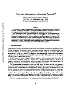
(23) Further details of the derivations are found in Appendix A. Even though the expectation in (19) is based on the code[i] word distribution, qd (d), only soft code symbols appear in (22) and (23). As a direct consequence of the formal DM framework, the codeword distributions need not to be computed. Only the posterior symbol-wise probability distributions are required. Further note that the covariance matrix Σ[i+1] a represents the estimation errors of the channel coefficients. The computation of (22) and (23) is summarized in Fig. 1-A.
L−1
B. Estimation of the Noise Covariance Matrix Distribution
l=Lp
[i] qa (a)
+
When updating the distribution of Σ−1 w , the distributions [i] and qd (d) are kept fixed. The minimum divergence is
438
IEEE JOURNAL ON SELECTED AREAS IN COMMUNICATIONS, VOL. 26, NO. 3, APRIL 2008
r ˜ d
r
[i]
[i+1]
Channel Estimation
[i] Σd
[i]
a
˜ d
Σ[i+1] a
Σd
[i]
[i+1] (Ω−1 w )
Noise Matrix Estimation
a[i]
[i] (Ω−1 w )
Σ[i] a
−1 B. Updating qσw −1 (Σw ) - noise matrix estimation.
A. Updating qa (a) - channel estimation.
where the right-hand-side of (25) has the form of a complex Wishart distribution3. −1 No prior distribution of Σ−1 w is available, thus p(Σw ) may be removed in (24). Inserting (25) into (24), it follows that is Wishart distributed as Σ−1 the random matrix Σ−1 w ∼ � � w �−1 � [i] WNc L + Nc + 1, B . The expectation of Σ−1 w is then given as � �−1 Ω[i+1] � Eq[i+1] {Σ−1 w w } = −1 Σw
[i] (Ω−1 w )
r ˜ [i] d ¯ k
[i+1]
γk
Interference Cancellation
[i]
Σd
Single-User Decoder for User k
[i+1] d˜k
Σ[i] a
a[i]
C. Updating qdk (dk ) - interference cancellation and single user decoding. Fig. 1. The modules for updating the distribution of the channel coefficient vector, the distribution of the noise covariance matrix, and the distribution of [i] the codewords of user k. Note that the code symbol covariance Σd can be [i] ˜ . obtained from E[i] [0], . . . , E[i] [L − 1] which are functions of d
achieved for the distribution [i+1]
qΣ−1 w
� −1 � � � Σw ∝ p Σ−1 w � � � �� · exp Eq[i] Eq[i] log p(r|a, d, Σ−1 , (24) w ) a
� � � � ��� exp Eq[i] Eq[i] log p r|a, d, Σ−1 w a d � � � −1 L [i] (25) ∝ |Σw | exp −tr Σ−1 w B with B [i] �
r[l] − S[l]Dp [l]a[i]
�� �H r[l] − S[l]Dp [l]a[i] �
l=0
+ +
H H S[l]Dp [l]Σ[i] a D p [l] S[l]
L−1 �
�� � � ˜ [i] [l]a[i] H ˜ [i] [l]a[i] r[l] − S[l]D r[l] − S[l]D
l=Lp
�−1
� � � [i+1] qσ−2 (σ −2 ) ∝ (σ −2 )LNc exp −σ −2 tr B [i] ,
,
(27)
(28)
where again the prior distribution is not available. With B [i] given in (26), the expectation of σ −2 is then �
Eq[i+1] σ
� −2
σ−2
� =
tr{B [i] } LNc + 2
�−1 .
(29)
C. Estimation of the Codeword Distributions Similar to (10) and (11), the optimization of the divergence (14) with respect to qdk (dk ), while keeping the distributions [i] [i] [i] [i] qa (a), qΣ− 1 (Σ−1 w ) and qdk¯ (d) = j�=k qdj (dj ) fixed, gives w the update rule [i+1]
qdk
[i+1]
(dk ) = qdk,c (dk,c ) ∝ p(dk ) � � �� � � � ��� · exp Eq[i] Eq[i] Eq[i] log p r|a, d, Σ−1 . (30) w −1 Σw
Lp −1��
B [i] L + Nc + 1
where B [i] is determined in (26). The computation of (27) is summarized in Fig. 1-B. Simpler expressions are obtained for white Gausian noise. When Σw represents the covariance matrix of a white = diag{σ −2 , . . . , σ −2 }, Gaussian noise vector with Σ−1 w −2 the reciprocal variance σ is chi-square distributed [34] as σ −2 ∼ χ2LNc +2 . The corresponding probability density function is given by
d
similarly to (7). To compute the exponential term in (24), we compute the expectation of (16) with respect to the given [i] [i] distributions qa (a) and qd (d). The expectation with respect [i] to qd (d) makes use of the results from (17) and (18), while [i] the marginalization with respect to qa (a) exploits the results from (22) and (23). It follows that
�
d¯ k
a
The prior distribution of dk,c ∈ Ck in (30) is a uniform distribution. Thus, � L−1 � [i+1] [i+1] qdk,c (dk,c ) ∝ exp dk [l]γk [l] for dk,c ∈ Ck , l=Lp
(31)
+ S[l]E [i] [l]A[i] (A[i] )H E [i] [l]H S[l]H [i] H H + S[l]E [i] [l]Diag{Σ[i] a }E [l] S[l] H ˜ [i] H ˜ [i] [l]Σ[i] + S[l]D a D [l] S[l]
� (26)
3 If the pdf of a complex random matrix A p×p that is symmetric and positive definite can be written as fA (A) ∝ |A|n−p−1 exp[−tr{V −1 A}], where n ≥ p and Vp×p is a constant matrix, the matrix A is said to be complex Wishart distributed as A ∼ Wp (n, V ); the expectation of A is nV [34].
HU et al.: A DIVERGENCE MINIMIZATION APPROACH TO JOINT MULTIUSER DECODING FOR CODED CDMA
[i+1]
and qdk
TABLE I U PDATE SCHEDULING SCHEMES FOR THE DM RECEIVERS .
[i+1]
(dk ) = qdk,c (dk,c ) = 0 for dk,c �∈ Ck , where
[i+1] γk [l]
� 2Re
−
K
��
[i] ak
�∗
� �−1 sk [l] Ω[i] r[l] w
DM1
H
� �−1 � �∗ [i] [i] [i] sj [l] d˜j [l] ak aj sk [l]H Ω[i] w
DM2
j=1 j�=k
−
DM3
K � K
� �∗ [i] [i+1] [i+1] [i+1] d˜j [l]λj uj � j uj � k
j=1 j � =1 j�=k
DM4
�� � �−1 · sk [l]H Ω[i] s [l] j w ��� � � �−1 � ∗ [i] [i] H = 2Re ak sk [l] Ωw � K �� K K �−1 [i] [i] [i]∗ ak · r[l] − ·sj [l]aj d˜j [l] − j=1 j � =1 j�=k
j=1 j�=k [i+1] [i+1] uj � j
· sj [l]λj
��� � �∗ [i+1] [i] uj � k . (32) d˜j [l]
The structure of (32) is that of interference cancellation, followed by linear filtering. Details of the derivations for (31) and (32) are found in Appendix B. Conceptually, the probability distribution function of the codeword vector dk,c ∈ Ck is estimated. However, as a consequence of the formal DM framework, the computations of (15), (24) and (31) only require the soft code symbols defined in (17). This does not mean that the code constraints are ignored. In fact, the expression in (31) is proportional to the updated codeword distribution, and vectors that are not codewords have zero probability. Thus it follows that the code constraints are enforced in this scheme. (See also remarks to (10).) In order to compute the probabilities of the code symbols from (31), the BCJR algorithm may be applied [35], [36], [37]. [i+1] Note that d˜k [l] can be considered as a posterior soft codesymbol. When comparing the structure of (31) to the LogAPP algorithm in [36], [37] (called LogMAP therein) gives rise [i+1] to an interesting interpretation: the value γk [l] may be related to the L-value for dk [l] based on the “observation” [i+1] [i+1] [i+1] γk [l], i.e., γk [l] = 12 L(γk [l]|dk [l]). Using this and the well-known rules for conversion between L-values and soft-symbols, extrinsic soft code symbols can be defined in a straightforward manner. These will only be used in Section V for the purpose of comparison, since the formal DM framework dictates the use of posterior soft code symbols. After the last iteration, the estimates of the information bits are obtained by making hard decisions on the posterior information bit probabilities provided by the single-user decoders. The module for computing the soft code symbols is demonstrated in Fig. 1-C. The lower triangular matrix U [i+1] (introduced in (38) in [i+1] Appendix B) with elements uj � j is obtained by a singular value decomposition of the positive semi-definite�symmetric � [i+1]
439
H
error covariance matrix, Σaa = U [i+1] Λ[i+1] U [i+1] , � � [i+1] [i+1] denoting the diagonal with Λ[i+1] = diag λ1 , . . . , λK
qa (a) → qσ−2 (σ −2 ) → qd1 (d1 ) . . . → → qdK (dK ) → qa (a) → qσ−2 (σ −2 ) → → qd1 (d1 ) . . . qa (a) → qσ−2 (σ −2 ) → qa (a) → → qd1 (d1 ) → qa (a) → qd2 (d2 ) . . . qa (a) → qσ−2 (σ −2 ) → qd1 (d1 ) → → qa (a) → qσ−2 (σ −2 ) → qd2 (d2 ) . . . . qa (a) → qσ−2 (σ −2 ) → qa (a) → → qd1 (d1 ) → qa (a) → qσ−2 (σ −2 ) → → qa (a) → qd2 (d2 ) . . .
matrix of the eigenvalues. The last term in (32), relying on singular value decomposition, is a correction term to the interference cancellation process, originating from the channel estimation covariance matrix, i.e., the corresponding estimation error. Since the correction is comparatively minor, becoming negligible after only a few iteration, it can comfortably be omitted without noticeable performance penalties.
D. Scheduling, Initialization, and Complexity A family of iterative DM receivers can be obtained by conducting the updates for the channel coefficients, the noise covariance matrix and the soft code symbols of the users according to different update schedules. No analytical approach for determining the optimum scheduling order has yet been proposed. In this paper, we evaluate the performance of the four different update schedules listed in Table I by means of Monte Carlo simulations. Although all four receivers are guaranteed to converge, they may converge to different stationary points, leading to different performance in terms of bit error rate (BER). The performance of the four DM receivers is considered in Section V. The computational complexity for the channel estimation (CE), the noise variance estimations (NE) and the interference cancellation (IC) are of the order OCE (K 3 ), ONE (Nc2 ) and OIC (K 3 ), respectively. For each of the evaluated schemes in Table I the corresponding complexity for one stage based on module activations (CE, NE and IC) are listed in Table II. For example, for the DM1 receiver, CE is activated once, NE is activated once and IC is activated K times per stage. The performance of the DM receivers depend on initializations and thus, it is important to initialize the iterative process properly. A reasonable compromise is to let the initial channel coefficient estimates be determined by a linear leastsquares estimator based on the pilot symbols. To get an initial estimate of the input probabilities to the single-user decoders, a decorrelating filter is applied to the received observation vector. Estimates can also be obtained using simple matched filtering, resulting in some loss of performance. Together with the initial estimates of the channel coefficients, the initial input probabilities are found. Similarly, an initial estimate of the noise covariance matrix is determined from (26) and (27), given the initial channel coefficient estimates and initial symbol probabilities.
440
IEEE JOURNAL ON SELECTED AREAS IN COMMUNICATIONS, VOL. 26, NO. 3, APRIL 2008
TABLE II M ODULE ACTIVATIONS PER STAGE . (CE: CHANNEL ESTIMATION , NE: NOISE COVARIANCE ESTIMATION , IC: INTERFERENCE CANCELLATION )
DM1 DM2 DM3 DM4
CE 1 K +1 K 2K
NE 1 1 K K
IC K K K K
E. Interpretations and Relations to Prior Art In this section we interpret our resulting joint channel estimation and decoding receiver algorithm, and we compare it to the receiver structures in [24], which we consider the current state-of-the-art. As mentioned above, the receiver in [24] is constructed based on three component parts; namely a channel estimator, an interference cancellation multiuser detector, and a bank of single-user APP channel decoders. Each component is designed independently based on the statistics of the inputs. Thus, no overall holistic framework is applied. The designs are based on the following assumptions. The thermal noise is zero-mean additive white Gaussian noise with known variance σ 2 ; the channel coefficient vector is zero-mean Gaussian with diagonal covariance matrix Σa ; only the code-symbol distributions are updated over iterations. With these assumptions, the channel coefficient vector is estimated based on LMMSE filtering as follows, a[i+1] =
L−1
� �−1 ˜ [i] [l]H S[l]H B [i] [l] Σa D r[l] ce
(33)
l=0 H ˜ [i] H ˜ [i] B [i] ce [l] = S[l]D [l]Σa D [l] S[l]
+ S[l]E [i] [l]Σa E [i] [l]H S[l]H + σ 2 I.
(34)
In addition, the multiuser detector is based on interference cancellation, following by linear filtering. The preferred linear filter is the unconditional, unbiased LMMSE filter defined as follows, � �∗ � �−1 [i+1] [i+1] [i] g ic,k [l]H = βk ak sk [l]H B ic (35) � L−1 1 [i] B ic = S[l]E [i] [l]A[i] (A[i] )H E [i] [l]H S[l]H L l=0 � + σ2 I , (36) where βk is a normalization constant to ensure an unbiased estimate. In contrast, our receiver algorithm is based on updating the distribution functions for the channel coefficient vector, the inverse noise covariance matrix, and the codewords. The holistic approach ensures that all statistical parameters are included. The estimation of the channel coefficient vector is described by (22) and (23), where the expression for the mean vector in (22) has the same structural format as the LMMSE estimate in (33). However, the inverse matrix filters in the two cases are different. Consider the last four terms of (26) together with (27). The first term is an estimate of the residual interference covariance matrix, e.g., thermal noise and residual multiple-access interference, while the remaining three terms
are estimation error covariance matrices caused by the channel coefficient vector, the codewords and the combined effects of the two. Compared to (26), the filter in (34) comprises only three of these terms. Since the channel coefficient vector distribution is not updated, one term is missing and the error covariance matrix Σa is constrained to be diagonal, making two of the remaining terms less accurate than the corresponding terms in (26) in our approach. More importantly, the covariance matrix of the residual interference is estimated as the first term in (26). With perfect cancellation the residual interference is nothing but the thermal noise; however, a significant level of residual multiple access interference is present in the early iterations. This residual interference is accounted for in (26) with only minor additional complexity as compared to (34), where only the effect of the thermal noise is accounted for. For the estimation of the codeword symbol-wise inputs to the APP channel decoders described by (32), the postcancellation linear filter has again the same structural format as the LMMSE filter in (35). Again however, the inverse matrix filters in the two cases are different. For our case in (32) the inverse matrix filter is in fact the same filter as was used for channel estimation, and thus, no additional complexity is introduced. Conversely, the filter in (36) is different from the filter in (34). In this case the filter in (36) has only two of the four terms in (26). As before, the most important difference is the use of an estimate of the residual interference in (26) in place of the diagonal covariance matrix of the thermal noise used in (36). Another significant difference between the two approaches is that the single user decoders in the DM receivers output posterior probabilities, while the similar structures in [24], as well as in [20], [22], [23] output extrinsic probabilities. As previously mentioned, the exchange of extrinsic probabilities follows from arguments of BP. In contrast, the formal DM framework investigated here justifies the posterior probability output from the single user decoders. V. S IMULATION RESULTS In this section we evaluate the performance of the proposed DM receivers by means of Monte Carlo simulations. In particular, we examine the four update schedules specified in Table I. The system model detailed in Section II is considered. Within the model, all users apply the same rate Rc = 1/2 terminated convolution codes with generators (5, 7)8 . The generated codewords have length Lc = 320 code symbols, corresponding to information sequences of length M = 158 information symbols. Random signature sequences of length Nc = 8 chips are assigned to the users. Each codeword is multiplexed with Lp random pilot symbols and each block of L = Lc + Lp symbols is transmitted through a block fading channel. The effective signal-to-noise ratio is defined as Eb /N0 = L/(Lc Rc ) · Es /N0 , where Es is the energy per code symbol and Eb is the energy per information bit. All the users have the same Eb /N0 . We assume additive white Gaussian noise with variance σ 2 = 1. The iterative process is terminated after 10 stages, which was found to be sufficient (see e.g. Fig. 4).
HU et al.: A DIVERGENCE MINIMIZATION APPROACH TO JOINT MULTIUSER DECODING FOR CODED CDMA
441
100
100
10−1
SU DM1 DM2 DM3 DM4 DM3
BER
BER
10−1
(↓) (↓) (↓) (↓) (↑)
10−2
10−3
SU DM3 DM3 DM3 DM3
4
6
8
Lp =4 Lp =5 Lp =6 Lp =7
10−2
10
12 Eb /N0 [dB]
14
16
18
20 10−3
Fig. 2. Averaged BER performance of the DM3 receiver for K = 32 users for an increasing number Lp of pilot symbols.
10
8
6
12 Eb /N0 [dB]
16
14
18
20
Fig. 3. Averaged BER performance of the DM receivers with different update schedules for K = 32 users. The users are updated in an increasing (↑) or a decreasing (↓) order of their estimated channel coefficients. 100 SU DM1 DM2 DM3 DM4 DM3
10−1
(↓) (↓) (↓) (↓) (↑)
BER
For our examples, the averaged BER performance BER is obtained by averaging the BER over all users, and where appropriate, it is compared to the performance of a singleuser (SU) system with known channel coefficients and known noise variance. The particular order of updating users also influences the performance. The best user schedule is based on sorting users in descending order according to estimated channel coefficients, where the strongest user is processed first. For comparison, we also consider a user update schedule based on sorting users in ascending order according to estimated channel coefficients. In Fig. 2, the averaged BER performance of the DM3 receiver is plotted for K = 32 users as a function of Eb /N0 , and with an increasing number of pilot symbols. As the number of pilot symbols increases from Lp = 4 to Lp = 6, the BER of the DM3 receiver approaches SU performance. No additional improvements can be observed when more than 6 pilot symbols are employed. Therefore, we choose Lp = 6 in the following examples. The total transmission overhead due to this number of pilot symbols is Lp /L ≈ 1.8%. In Fig. 3 and Fig. 4, we compare the performance of the DM receivers with different scheduling schemes for K = 32 users. The four receivers update users according to descending estimated channel coefficients. For comparison, we also consider the DM3 receiver with a user schedule based on ascending estimated channel coefficients. We observe in Fig. 3 that the DM3 receiver estimating the strongest users first outperforms the DM3 receiver estimating the weakest users first. We also observe that all the simulated receivers perform close to the SU case with the DM4 receiver exhibiting the best performance. The DM3 and DM4 receivers have better BER performance than the DM1 and DM2 receivers, since the channel estimation and the estimation of the noise covariance matrix are performed more often for each stage. However, the DM3 and DM4 receivers have higher complexities per stage as compared to the DM1 and DM2 receivers. In Fig. 4, the BERs of the receivers are shown as a function of the number of stages. The improvement on BER
4
10−2
10−3
1
2
3
4
5 6 Number of stages
7
8
9
10
Fig. 4. Averaged BER performance of the DM receivers with different updating schedules versus number of stages for K = 32 users at Eb /N0 = 16 dB. The users are updated in an increasing (↑) or a decreasing (↓) order of their estimated channel coefficients.
is marginal after 5-6 stages for the DM3 and DM4 receivers and after 9-10 stages for the DM1 and DM2 receivers. The BER of the DM3 receiver and the DM4 receiver improves at a similar rate. However, as the DM3 receiver is less complex than the DM4 receiver, we consider the DM3 receiver in the following examples. In Fig. 5, we compare DM3 receivers based on APP feedback as dictated by the DM framework, extrinsic feedback as suggested in [20], [22], and hard-decision feedback [28]. We observe that for K = 32 users the DM3 receiver with extrinsic feedback performs considerably worse than the receivers based on hard-decision and APP feedback, respectively. Thus, both the theoretical framework and the simulation results support that posterior probabilities rather than extrinsics should be used for computing the soft symbols. The DM3 receiver with
442
IEEE JOURNAL ON SELECTED AREAS IN COMMUNICATIONS, VOL. 26, NO. 3, APRIL 2008
100
100 SU DM3 (known a, σ 2 ) DM3 (known σ 2 ) DM3 (known a) DM3 (all unknown) 10−1
DM3 (one σ 2 update only)
BER
BER
10−1
10−2
10−2 SU DM3 (extrinsc) DM3 (hard) DM3 (APP)
10−3
4
8
6
10
12 Eb /N0 [dB]
14
18
16
20
10−3 24
26
28
30
32
34
36
38
40
42
44
46
K
Fig. 5. The averaged BER performance of the DM3 receiver with APP, extrinsic and hard-decision feedback, respectively, for K = 32 users. The users are sorted in a descending (↓) order of estimated channel coefficients.
Fig. 7. The averaged BER performance of the DM3 receiver under different conditions of known channel state information, as a function of number of users K at Eb /N0 = 16 dB. The users are sorted in a descending (↓) order of estimated channel coefficients.
100 SU DM3 (extrinsic) DM3 (hard) DM3 (APP) LMMSE [24] SAGE-based [31] SISO-SAGE [32] SAGE [29]
BER
10−1
receiver, enjoying a notably more graceful BER degradation. The SAGE-based receiver performs slightly worse, but enjoys a similarly graceful BER degradation. The SAGE receiver is competitive up to K = 32, after which it suffers rapid degradation at the same rate as the DM3 with hard decisions. Note that the performance of the LMMSE receiver in [24] is obtained by assuming perfect noise variance, while in the DM receiver, no prior information about the noise variance is available.
10−2
10−3 24
26
28
30
32
34
36
38
40
42
44
46
K
Fig. 6. The averaged BER performance as a function of the number of users K at Eb /N0 = 16 of the DM3 receivers with extrinsic, hard, and APP decision feedback, respectively, the LMMSE receiver [24], the SAGE-based receiver [31], the SISO-SAGE receiver [32], and the SAGE receiver [29]. The users are sorted in a descending (↓) order of estimated channel coefficients.
hard decisions performs slightly worse than the receiver with APP feedback. In Fig. 6, we compare the BER performance of the DM3 receivers and other related receivers [24], [29], [31], [32] as a function of the system load in terms of numbers of users at Eb /N0 = 16 dB. The DM3 receiver with extrinsic feedback is not competitive. Even at K = 24 users, the receiver is not able to provide SU performance. The DM receivers with harddecision feedback, with APP feedback, the LMMSE receiver [24], the SAGE-based receiver [31], and the SISO-SAGE [32] exhibit close to SU BER performance up to K = 34 users. For K > 34 users, the performance of the DM3 with hard decisions and the SISO-SAGE deteriorate rapidly. Similar behavior is observed for the DM3 receiver and the LMMSE
In Fig. 7, we investigate the BER performance of the DM3 receiver under different conditions in terms of numbers of users at Eb /N0 = 16 dB. It is shown that the BER performance of the receiver that updates the noise variance in the iterative process is always better than the one of the receiver that does not update the noise variance (The noise variance is either assumed to be known or estimated only once.). Although curious at first, the behavior is to be expected. With an increasing number of users in the system, the amount of multiple-access interference (MAI) is increasing. Beyond a certain level of MAI, the interference cancellation process is overwhelmed, resulting in an increasing level of residual interference. The residual interference can be considered as additional additive noise, which can be estimated and accounted for together with the additive white Gaussian noise, leading to better performance. Therefore, it is very important to include the noise variance estimation in the iterative process. Since we assume σ 2 = 1 in the cases considered here, the noise covariance matrix is an identity matrix. The estimated noise variance as a function of the number of stages is plotted in Fig. 8 for K = 32 and different Eb /N0 . At the first few stages, a significant part of the estimated noise variance comes from the residual interference. As more stages are performed, there is less residual interference left. The estimated noise variance finally converges to the true noise variance after 9 to 10 stages.
HU et al.: A DIVERGENCE MINIMIZATION APPROACH TO JOINT MULTIUSER DECODING FOR CODED CDMA
100
443
in
DM3 12dB DM3 16dB DM3 20dB
[i]
[i]
˜ [l]ar[l]H ˜ [l]H S[l]H − S[l]D r[l]r[l]H − r[l]aH D � � + S[l]A Eq[i] d[l]d[l]H AH S[l]H
estimate of σ 2
d
[i]
[i]
˜ [l]H S[l]H − S[l]D ˜ [l]ar[l]H = r[l]r[l]H − r[l]aH D ˜ [i] [l]d ˜ [i] [l]H AH S[l]H + S[l]Ad
10
+ S[l]AE [i] [l]E [i] [l]H AH S[l]H , which leads to (19). It follows that (15) is
1
� �� �−1 qa[i+1] (a) ∝ p(a) exp −tr Ω[i] w 1
2
4
3
5 6 no. of stages
7
8
9
10
·
Fig. 8. The estimated noise variance of the DM3 receiver at different stages for K = 32 users, at Eb /N0 = 12, 16, 20 dB. The users are sorted in a descending (↓) order of estimated channel coefficients.
�L p −1 (r[l]−S[l]Dp [l]a)(r[l]−S[l]Dp [l]a)H
+
A formal optimization framework based on divergence minimization has been proposed for the systematic design of low-complexity iterative receivers performing iterative joint channel estimation, noise covariance estimation, multiuser interference cancellation using soft code symbols and single user APP decoding. As a consequence of the holistic approach, the framework inherently accounts for the covariance of all estimated parameters, as well as the highly nonlinear channel code constraints. Previously known receivers developed based on EM/SAGE algorithms and variational free energy minimization are contained within the framework as special cases of the required factorized auxiliary distribution function. It follows that well-known receiver structures can be formally justified and generalized within the divergence minimization paradigm. A detailed comparison to the receiver structure in [24] demonstrated the versatility and generality of the framework.
[i]
From (16), the expectation in (19) with respect to qd (d) is determined as follows, �� � � �−1 �� −1 e Eq −1 Eq[i] log p(r|a, d, Σw ) ∝ −tr Ω[i] w d
�L p −1 · (r[l]−S[l]Dp [l]a)(r[l]−S[l]D p [l]a)H
d
� L−1
r[l]r[l]H − r[l]aH D[l]H S[l]H
l=Lp
− S[l]D[l]ar[l]H + S[l]D[l]aaH D[l]H S[l]H
��� .
Exchanging the order of summation and expectation for the last four terms on the right-hand-side, the expectation results
���
L−1
[i]
[i]
H
(S[l]AE [l])(S[l]AE [l])
,
l=Lp
leading to (21), (22), and (23). The expectation in (25), leading to (26) is determined in a similar manner.
B. Derivations for the Codeword Distributions Using the results in (17) and (18) for codeword marginals and the results in (22) and (23) for channel coefficient vector marginals, we can compute the marginalization in (31) as follows ��� � � � ) EΣ[i] Eq[i] Eq[i] log p(r|a, d, Σ−1 w w
a
∝ −tr
A. Derivations for Estimating the Channel Coefficient Vector Distribution
+ Eq[i]
+
e
A PPENDIX
l=0
˜ [i] [l]a)(r[l]−S[l]D ˜ [i] [l]a)H (r[l]−S[l]D
l=Lp
VI. C ONCLUSIONS
Σw
l=0 L−1
��
d¯ k
Ω[i] w
�−1 L−1 �� � ˜ [i] [l]a[i] r[l]−S[l]D k l=Lp
� � ˜ [i] [l]a[i] H · r[l]−S[l]D k
�
� [i] [i] ˜ [i] H H ˜ + S[l]Dk [l]Σa D k [l] S[l] , (37)
˜ [i] [l](I −diag{ek })+D[l]diag{ek } and ek ˜ [i] [l] = D where D k is a unit vector with element k equal to 1. Terms independent of dk [l], l = Lp , . . . , L − 1 are discarded in (37). The compact expression in (31) is obtained from (37) by expanding the matrix-vector multiplications, and discarding terms irrelevant for determining the codeword distribution for user k. Exploiting the properties of the trace operator, and decomposing the error covariance matrix, the trace operation can be eliminated. In particular, since the symmetric error covariance matrix Σ[i] a is always positive semi-definite we can em[i] [i] [i] H ploy a singular value decomposition, Σ[i] a = U Λ (U ) ,
444
IEEE JOURNAL ON SELECTED AREAS IN COMMUNICATIONS, VOL. 26, NO. 3, APRIL 2008
to obtain the last term in (32) as follows � � L−1 [i] [i] ˜ [i] H −1 H ˜ tr (Ω[i] D ) S[l] D [l]Σ [l] S[l] k k w a l=Lp
� L−1 −1 ˜ [i] [l]U [i] Λ[i] (U [i] )H = tr (Ω[i] ) S[l]D w k l=Lp
� [i] H H ˜ · Dk [l] S[l]
=
L−1
� ˜ [i] [l]H S[l]H (Ω[i] )−1 S[l] tr (U [i] )H D k w
l=Lp [i]
�
˜ [l]U [i] Λ[i] ·D k ∝e
L−1
� [i] H H [i] [i] � (38) dk [l]2Re (uk ) sk [l](Ω[i] )−1 sj uj λj
l=Lp
j�=k
[i]
where uk is the kth column of eigenvector matrix U [i] , and λ[i] is the jth eigenvalue of the diagonal matrix Λ[i] . R EFERENCES [1] T. R. Giallorenzi and S. G. Wilson, “Multiuser ML sequence estimator for convolutionally coded asynchronous DS-CDMA systems,” IEEE Trans. Commun., vol. 44, pp. 997–1008, Aug. 1996. [2] H. V. Poor, “Iterative multiuser detection,” IEEE Signal Processing Mag., vol. 21, no. 1, pp. 81–88, Jan. 2004. [3] M. Moher, “An iterative multiuser decoder for near-capacity communications,” IEEE Trans. Commun., vol. 46, pp. 870–880, July 1998. [4] M. C. Reed, C. B. Schlegel, P. D. Alexander, and J. A. Asenstorfer, “Iterative multiuser detection for CDMA with FEC: Near-single-user performance,” IEEE Trans. Commun., vol. 46, pp. 1693–1699, Dec. 1998. [5] J. Boutros and G. Caire, “Iterative multiuser joint decoding: Unified framework and asymptotic analysis,” IEEE Trans. Inf. Theory, vol. 48, pp. 1772–1793, July 2002. [6] P. D. Alexander, A. J. Grant, and M. C. Reed, “Iterative detection in code-division multiple-access with error control coding,” Euro. Trans. Telecomms., vol. 9, pp. 419–425, Sept. 1998. [7] X. Wang and H. V. Poor, “Iterative (Turbo) soft interference cancellation and decoding for coded CDMA,” IEEE Trans. Commun., vol. 47, pp. 1046–1061, July 1999. [8] H. El Gamal and E. Geraniotis, “Iterative multiuser detection for coded CDMA signals in AWGN and fading channels,” IEEE J. Sel. Areas Commun., vol. 18, pp. 30–41, Jan. 2000. [9] G. Caire, R. M¨uller, and T. Tanaka, “Iterative multiuser joint decoding: Optimal power allocation and low-complexity implementation,” IEEE Trans. Inf. Theory, vol. 50, pp. 1950–1972, Sept. 2004. [10] P. H. Tan and L. K. Rasmussen, “Asymptotically optimal nonlinear MMSE multiuser detection based on multivariate Gaussian approximation,” IEEE Trans. Commun., vol. 54, pp. 1427–1438, Aug. 2006. [11] H. A. Bethe, “Statistical Theory of Superlattices,” in Roy. Soc. London, 1935, p. 552. [12] J. S. Yedidia, W. T. Freeman, and Y. Weiss, “Generalized belief propagation,” Advances in Neural Information Processing Systems (NIPS), vol. 13, pp. 689–695, Dec. 2000. [13] J. S. Yedidia, W. T. Freeman, and Y. Weiss, “Constructing free-energy approximations and generalized belief propagation algorithms,” IEEE Trans. Inf. Theory, vol. 51, no. 7, pp. 2282–2312, July 2005. [14] P. H. Tan, Simplified Graphical Approaches for CDMA Multi-user Detection, Decoding and Power Control, Ph.D. thesis, Department of Computer Science and Engineering, Chalmers University of Technology, Sweden, 2005. [15] P. H. Tan and L. K. Rasmussen, “Belief propagation for coded multiuser detection,” in Proc. IEEE Int. Symp. Inf. Theory, Seattle, Washington, USA, July 2006, pp. 1919–1923. [16] H. Attias, “Inferring parameters and structure of latent variable models by variational Bayes,” in Proc. 15th Conf. on Uncertainty in Artificial Intelligence, 1999.
[17] A. Dempster, N. Laird, and D. Rubin, “Maximum likelihood from incomplete data via the EM algorithm,” J. Royal Statist. Soc., Ser. B, vol. 39, pp. 1–38, Jan. 1977. [18] M. Beal, Variational Algorithms For Approximate Bayesian Inference, Ph.D. thesis, Gatsby Computational Neuroscience Unit, London’s Global University, UK, 2003. [19] L. P. B. Christensen and J. Larsen, “On data and parameter estimation using the variational Bayesian EM-algorithm for block-fading frequence-selective MIMO channels,” in Proc. IEEE Int. Conf. on Acoustics, Speech and Signal Processing, 2006, vol. 4, pp. 465–468. [20] D. D. Lin and T. J. Lim, “A variational free energy minimization interpretation of multiuser detection in CDMA,” in Proc. IEEE Global Telecomms. Conf., Nov. 2005, pp. 1570–1576. [21] J. A. Fessler and A. O. Hero, “Space-alternating generalized expectation-maximization algorithm,” IEEE Trans. Signal Processing, vol. 42, pp. 2664–2677, Oct. 1994. [22] M. Kobayashi, J. Boutros, and G. Caire, “Successive interference cancellation with SISO decoding and EM channel estimation,” IEEE J. Sel. Areas Commun., vol. 19, pp. 1450–1460, Aug. 2001. [23] A. Lampe, “Iterative multiuser detection with integrated channel estimation for coded DS-CDMA,” IEEE Trans. Commun., vol. 50, pp. 1217–1223, Aug. 2002. [24] J. Wehinger and C. F. Mecklenbr¨auker, “Iterative CDMA multiuser receiver with soft decision-directed channel estimation,” IEEE Trans. Signal Processing, vol. 54, pp. 3922–3934, Oct. 2006. [25] A. J. Grant P. D. Alexander, “Iterative channel and information sequence estimation in CDMA,” in Proc. IEEE 6th Int. Symp. on Spread-Spectrum Tech. & Appli, New Jersey, USA, Sept. 2000, pp. 593–597. [26] H. Li, S. M. Betz, and H. V. Poor, “Performance analysis of iterative channel estimation and multiuser detection in multipath DS-CDMA channels,” IEEE Trans. Signal Processing, vol. 55, no. 5, pp. 1981– 1993, May 2007. [27] A. Kocian and B. H. Fleury, “EM-based joint data detection and channel estimation of DS-CDMA signals,” IEEE Trans. Commun., vol. 51, pp. 1709–1720, Oct. 2003. [28] A. Kocian, I. Land, and B. H. Fleury, “Optimal weighting of softinformation in a SAGE-based iterative receiver for coded CDMA,” in Proc. IEEE Global Telecomms. Conf., Nov. 2005, vol. 3, pp. 1555–1559. [29] A. Kocian, I. Land, and B.H. Fleury, “Joint channel estimation, partial successive interference cancellation, and data decoding for DS-CDMA based on the SAGE algorithm,” IEEE Trans. Commun., vol. 55, no. 6, pp. 1231–1241, June 2007. [30] E. Chiavaccini and G. M. Vitetta, “MAP symbol estimation on frequency-flat rayleigh fading channels via a Bayesian EM algorithm,” IEEE Trans. Commun., vol. 49, pp. 1869–1872, Nov. 2001. [31] B. Hu, I. Land, R. Piton, and B. H. Fleury, “Iterative SAGE-based receivers for synchronous coded DS-CDMA,” Proc. the 66th SemiAnnual IEEE Vehicular Tech. Conf., 2007. [32] B. Hu, A. Kocian, R. Piton, A. Hviid, B. H. Fleury, and L. K. Rasmussen, “Iterative joint channel estimation and successive interference cancellation using a SISO-SAGE algorithm for coded CDMA,” in Proc. IEEE 38th Asilomar Conference on Signals, Systems & Computers, Pacific Grove, California, Nov. 2004, pp. 622–626. [33] T. M. Cover and J. A. Thomas, Elements of Information Theory, John Wiley and Sons, 1991. [34] A. K. Gupta and D. K. Nagar, Matrix Variate Distributions, Chapman & Hall/CRC, 2000. [35] L. R. Bahl, J. Cocke, F. Jelinek, and J. Raviv, “Optimal decoding of linear codes for minimizing symbol error rate,” IEEE Trans. Inf. Theory, vol. 20, pp. 284–287, Mar. 1974. [36] J. Hagenauer, “Iterative decoding of binary block and convolutional codes,” IEEE Trans. Inf. Theory, vol. 42, pp. 429–445, Mar. 1996. [37] P. Robertson, P. Hoeher, and E. Villebrun, “Optimal and sub-optimal maximum a posteriori algorithms suitable for turbo decoding,” Euro. Trans. Telecomms., vol. 2, pp. 119–125, Mar. 1997.
HU et al.: A DIVERGENCE MINIMIZATION APPROACH TO JOINT MULTIUSER DECODING FOR CODED CDMA
Bin Hu is currently pursuing a Ph.D. degree in Wireless Communications at Aalborg University, Aalborg, Denmark. She received her M.Sc. degree in Digital Communications from Aalborg University, Denmark in 2003 and her B.Sc. degree in Electronics Engineering from Jilin University, Changchun, China in 2000, respectively. Her research interest is iterative algorithm design for channel estimation, interference cancellation, equalization and multiuser decoding in wireless communication systems.
Ingmar Land is a Research Fellow at the University of South Australia, Australia, since 2007, and he has been an Assistant Professor at Aalborg University, Denmark, since 2005. He received his Dr.-Ing. degree at the University of Kiel, Germany, in 2004, and he studied electrical engineering at the Universities of Ulm and Erlangen-N¨urnberg, Germany, where he received his Dipl.-Ing. degree in 1999. Ingmar Land is a Member of the IEEE and a member of the IEEE Information Theory and Communications Societies. His main areas of research are channel coding, iterative decoding, information theory, and multiuser decoding. Ingmar Land received the best paper award of the German Information Technology Society (ITG) in 2006, and he received the “Teacher of the Year” Award in Electronics and Information Technology, Aalborg University, in 2006.
Lars K. Rasmussen was born on March 8, 1965 in Copenhagen, Denmark. He got his M.Eng. in 1989 from the Technical University of Denmark, and his Ph.D. degree from Georgia Tech (Atlanta, Georgia, USA) in 1993. From 1993 to 1995, he was a Research Fellow at the University of South Australia (Adelaide, Australia). From 1995 to 1998 he was a Senior Member of Technical Staff with the Centre for Wireless Communications at the National University of Singapore (Singapore). From 1999 to 2002 he was an Associate Professor at Chalmers University of Technology (Gothenburg, Sweden), where he maintained a parttime appointment until 2005. He has held visiting positions at University of Pretoria, South Africa (1998), Southern Poro Communications, Australia (2001), and University of Aalborg, Denmark (2003,2004). Dr. Rasmussen is currently the leader of the Communications Signal Processing research group at the Institute for Telecommunications Research, University of South Australia, where his research interests include multiple user communications, iterative information processing, and adaptive modulation and coding. Prof. Rasmussen is a Senior Member of the IEEE, a member of the IEEE Information Theory and Communications Societies and served as Chairman for the Joint ACT/SA/Vic/NSW Chapter of the IEEE Information Theory Society 2004-2005. He was a member of organizing committees for the IEEE 2004 International Symposium on Spread Spectrum Systems and Applications held in Sydney, Australia, and the IEEE 2005 International Symposium on Information Theory held in Adelaide, Australia. He is also an associate editor for IEEE Transactions on Communications in the areas of iterative detection, decoding and ARQ. Prof. Rasmussen has published a total of more than 100 refereed journal and conference papers, and in 2004 Dr. Rasmussen was part of the successful bid for the ARC Communications Research Network (ACoRN), for which he is now the Network Convenor. Prof. Rasmussen is a co-founder of Cohda Wireless Pty Ltd, which was established in 2002 (incorporated 2003) from technology produced by researchers from the Institute for Telecommunications Research (ITR) at the University of South Australia.
445
Romain Piton is completing his Ph.D. degree at Motorola A/S, Aalborg, Denmark in collaboration with Aalborg University, Aalborg, Denmark. He received his M.Sc. degree in Digital Communication from Aalborg University, Denmark and also his Dipl.-Ing degree from the ”Ecole Sup´erieur d’Ing´enieurs en Electronique et Electrotechnique” (ESIEE) Paris, France, both in 2004. His research topics are in the area of wireless communication with a special emphasis on interference cancellation, iterative algorithm design, diversity techniques and narrow-band multiuser detection.
Bernard H. Fleury received the diploma in electrical engineering and mathematics in 1978 and 1990 respectively, and the doctoral degree in electrical engineering in 1990 from the Swiss Federal Institute of Technology Zurich (ETHZ), Switzerland. Since 1997 Bernard H. Fleury has been with the Department of Electronic Systems, Aalborg University, Denmark, as a Professor in Communication Theory. He is currently the Head of the Section Navigation and Communications of this department. Since April 2006 he has also been affiliated as a Key Researcher with ftw. Forschungszentrum Telekommunikation Wien, Austria, where he is the Manager of the Research Area Signal and Information Processing. In 1999 he was elected IEEE Senior Member. During 1978-85 and 1988-92 he was respectively a Teaching Assistant and a Research Assistant at the Communication Technology Laboratory and at the Statistical Seminar at ETHZ. In 1992 he joined again the former laboratory as a Senior Research Associate. Prof. Fleury’s general fields of interest cover numerous aspects within communication theory and signal processing, mainly for wireless communications. His current areas of research include stochastic modelling and estimation of the radio channel, especially for multiple-input multiple-output (MIMO) applications and in fast time-varying environments, and iterative information processing with focus on efficient, feasible advanced receiver architectures. He has authored and co-authored more than 70 publications in these areas. Prof. Fleury has developed with his staff a high-resolution method for the estimation of radio channel parameters that has found a wide application and has inspired similar estimation techniques both in academia and in industry.